Radial Trees in Tableau by Chris DeMartini

Radial-Tree-Feature-Image1.png

Before we get into it, I wanted to include a shameless plug for my fellow DataBlick'ers upcoming sessions at the Tableau Conference. Be sure to check them out if you are heading that way!


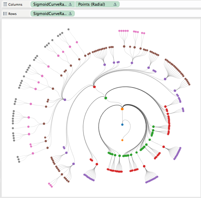
This is an incremental post to navigating your family tree from a few months back. This builds off of that visualization technique to manipulate the tree into a radial view. Also, as with the original, the tree is 100% dynamic and you can reset each node in the tree as the root node, toggle between tree views as well as change the API you are analyzing.


What is the benefit of a radial tree? As I discussed in my recent Tableau Fringe Festival presentation, it is really a give and take. Overall, it is probably easier to follow a path through a horizontal/vertical tree diagram. However, as your data volume and hierarchy levels increase, you will ultimately run out of space on your screen. That is where the radial tree can add value. With the root node as the center of the viz, and each level of the hierarchy increasing in diameter, you ultimately have more viz real estate to work with as you dig deeper into your hierarchy.


The use case I leveraged for this post is taking a look at the Tableau JS API class/object structure. I chose this in order to more easily navigate the Tableau JS API objects available to us all. I also incorporated the Flare API class structure for comparison purposes. Lastly, this effort was inspired by a similar D3 implementation.


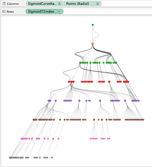
To arrive at the radial tree, I started with the vertical hierarchy tree, a carbon copy of the family tree post discussed above. From this point it was just a matter of taking this tree and manipulating it into a circle. Honestly, I spent way more time than needed trying to figure out how to do this with a whole new set of calculations. If it is not broken, don't fix it! Once I settled on leveraging my existing tree and just manipulating it into a radial version, I needed a total of five additional calculated fields to bend my vertical tree into a radial tree.


Calculation 1: A window table calculation to apply PI() across our data densification technique.

Radial Tree Pic 1


Calculation 2: A level of detail calculation that will return the maximum node placement across the entire population. This result is than applied to the same table calculation as our other fields. LOD made this so much easier!

Radial Tree Pic 2


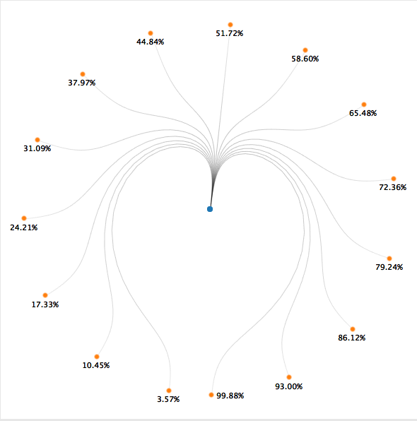
Calculations 3 and 4: This is the trickiest part. Leveraging our previous sigmoid curve function we are going to create x/y coordinates in a circle. One of the main things we need to know is where our points are in relation to one another. To figure this out, I used a percentage of maximum node technique. This is best described by the below images and I once again leveraged the handoff-map created by Joe Mako.

Radial Tree Pic 3aRadial Tree Pic 3b


In this example the left most node is closest to 0% and the right most node is closest to 100%. We adapt that to a circle implementation shown on the right, via the below calculations.

Radial Tree Pic 3c

Radial Tree Pic 4

Quick side note: While in the process of implementing these fields, I came across this result, not very meaningful, but reminded me of star wars a bit…

Radial Tree Pic 5


Calculation 5: This last calculation is just an adaptation of Jeffery Shaffer’s “Points” calculation, leveraging our radial field created above instead of our linear field.

Radial Tree Pic 6

From here we just need to place the respective calculations on their corresponding shelves and we now see our radial tree! Compare the two versions below and you will note identical use of our rows/columns shelves (inversed) between the two implementations.

Radial Tree Pic 7aRadial Tree Pic 7b

There have been a couple requests for the underlying excel files, you can download them here.

Alteryx Newbie Creates Dynamic Parameters in Tableau First Day by Jonathan Drummey

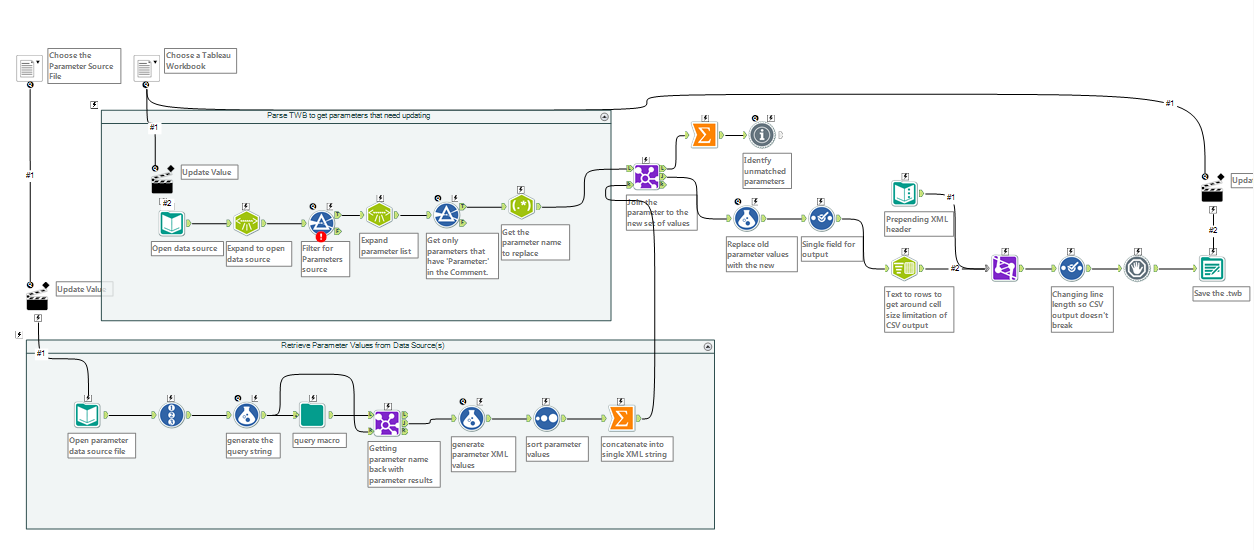
I am delighted and beyond honored to announce the first DataBlick post from the famed Jonathan Drummey.  In his first few hours following an introduction to Alteryx training he came up with an elegant solution to dynamic parameters in Tableau as described below.  Go Jonathan!

First, watch this 4 minute video on what an Alteryx newbie (yours truly) just did:

https://vimeo.com/jonathandrummey/alteryx-newbie-creates-dynamic-parameters-in-tableau

How this Came to Be

Yesterday most of the DataBlick staff were at an Alteryx training with friend Allan Walker:

https://twitter.com/datablick/status/637283689173377025

Though he's already and Alteryx Ace, Joe Mako was there to help us Tableau users make the translation to Alteryx and see what else he could absorb, and Allan Walker was there to sit in the corner working on his laptop and occasionally giggle like a schoolboy. (I think we'll get to see what he was up to at the Tableau Conference).

As I learned more about Alteryx through the day I came away incredibly impressed at its capabilities as a visual environment for manipulating & transforming data along with the attention the Alteryx developers have had for the "meta" aspects of working with data: we can visually inspect every step of the Alteryx pipeline and rewrite if need be, and we have the tools to build our own pipelines from the ground up.

I wanted to take Alteryx out for a drive to see what it could do and decided to look into the Tableau XML, in particular using Alteryx to dynamically update Tableau parameters. This is something I've worked on before (see Creating a Dynamic Parameter with a Tableau Data Blend) and last year at the Tableau Conference Bryan Brandow & Andy Kriebel demoed a solution that they'd built for Facebook with the same basic idea as my Alteryx one. The particular use case is one of the most requested ones for dynamic parameters, namely updating the parameter list as the data changes.

This morning I built a demo Tableau workbook and started building an Alteryx workflow. With about 5 hours of effort I learned some regex, figured out Tableau's XML structure, learned Alteryx's XML Parse tool, learned how to build an Alteryx macro, constructed the configuration file, built two Alteryx macros, and had a working prototype of a tool that opens up the Tableau workbook XML, queries the data source for the latest values of the selected parameters, and then writes out the new values to back to the workbook:

Screen Shot 2015-08-29 at 10.54.50 PM

One note on the configuration of this - besides the necessary parameter data source file that I described, the Tableau parameter has a comment field that indicates which query to pull data from:

Screen Shot 2015-08-29 at 11.23.59 PM

Now, I did have one advantage over your average Alteryx newbie and that is having Joe Mako in the room here at DataBlick HQ. I was pretty determined to build this myself, and at the same time I had some regex difficulties and building Alteryx macros were completely new so his help saved time reading help files and running Google searches. Thanks, Joe!

The macro is really a version 0.1 proof of concept, I haven't tested it out on multiple parameters in the same workbook, it issues more queries than it needs to, it only handles .twb files and not .twbx (Tableau Packaged Workbooks), and really needs to take advantage of Tableau's REST API so we can download all the workbooks at once from Tableau Server to update the parameters & republish them. And I must make the obligatory caveat that rewriting the XML is  totally unsupported by Tableau so if your workbook breaks then you're on your own. And maybe this'll all be moot depending on what Tableau announces in October. But in the meantime we've got yet another way to get more utility out of Tableau, I've got some updates to make, and I've got a whole bunch of new knowledge available to help out more people.

Here's the macro if you want to take a look at it yourself: update Tableau parameter v0.1.yxzp

Navigating your Family History in Tableau by Chris DeMartini

Context

A while back, I was talking to my mom about one of her passions, tracing the history of our family lineage. She has spent more time on this than I can really comprehend at this point and has traced our family all the way back to the 1600s (cheers to you mom!). During the discussion I asked her to show me my ancestor tree. She said no problem, and then printed out 23 pages of paper containing my ancestor tree, which she then taped together and laid out on the floor shown below.

Family Tree Pic 1

This does show my family tree, but I wondered if I could help my mom out with the following challenges presented by her genealogy software’s reporting limitations:

  • Generating the tree was a time consuming process. She had to print, tape and then find a place large enough to view the tree.
  • The size of the tree is not conducive to review, you literally have to walk several feet to review it (which is why you see my left foot twice in the above picture). Also, looking at more than one tree at a time would be extremely difficult and take up most of the floor space in the house.
  • The tree was static. She had to select a root, direction (ancestor/ descendant) and then print, tape, etc. Then repeat this for each root from which she wanted to view lineage.
  • Information was limited to what could fit in the box allocated to each person in the tree. The tree was 1 dimension, additional context cannot easily be added or modified.
  • And let’s face it, the tree print out is not very tree friendly (pun intended).

So, now that we know what we are trying to fix, how do we go about this. Obviously, I immediately started to see the value that Tableau and its interactive nature could bring to my mom’s research. We can address all the issues mentioned above just be leveraging Tableau’s native functionality and a few tricks.

The Viz

We are going to build two tree views in Tableau, an ancestor view and a descendant view of a dynamically selected root person. Within this post I will walk through building the ancestor tree (a binary tree), feel free to reach out if you want more information on how the descendant tree was built, but will leave that to the imagination for now.

First things first, the credits. I started this effort with two main inputs, (1) the node tree link diagram that was explained and created by Jeffery Shaffer and (2) the dynamic parameter posts that Nelson Davis recently went through. I rely on both of these to get to the family tree viz shown here. In addition to these, I also asked Allan Walker, Noah Salvaterra and Anya A’Hearn for general help and guidance along the way. Also, thanks again for lending your blog Anya!

Quickly on the underlying data format. For the most part it is the same overall setup as shown in the Hive plot post. Refer back to that (or the workbook itself) to dig into how the underlying data has been structured to support the visualization shown here.

One of the most important aspects of building the viz is how to place the various nodes within the viz. From there we will leverage Shaffer’s node tree link diagram with a tweak to place the curved lines in between our nodes. Everything will be based from the root node and built up or down from there.

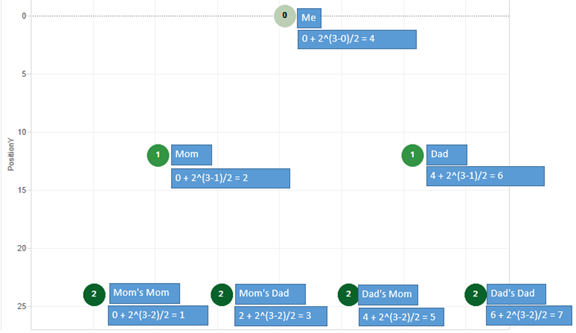
Onto to node placement already! The Y-axis of the node placement is simpler for this use case. We are going to assign a Y value based on the node’s generation. Root node is generation 0, parents are generation 1, and grandparents are generation 2 and so on. Then in order to leverage Shaffer’s curve equation for our tree we multiply the generation by 12.

Family Tree Pic 2

Now the hard part, where do we put the nodes on the X-axis. I have two solutions for this, one for ancestor where we have two and only two parent nodes and another for descendants where we have 1 to N child nodes. As mentioned, we will walk through the ancestor tree view in this post.

When examining the ancestor tree, we see that each generation has two to the power of N worth of nodes. For example:

  • Generation 0 (Root Node) is 2^0 = 1 node
  • Generation 1 (Root’s Parents) is 2^1 = 2 nodes
  • Generation 2 (Root’s Grandparents) is 2^2 = 4 nodes
  • Generation N is 2^N nodes

So our tree width needs to increase by this factor as we continue to add generations to the tree. I also enforced a rule that all females will be on the left side and all males will be on the right. As a result of this rule, we need to keep track of how many males are in the lineage of the specific node we are trying to place. Here is a table breaking down how I went about the calculation for Position X. Disclaimer: the [XPosStart] and the generation counter ([A]) were both created outside of Tableau using a recursive CTE in SQL Server (reach out if you want the nitty gritty on this). If you have successful feedback on the way to implement this recursive calculation step in Tableau, I’ll have a beer waiting for you at TCC15. I am sure it can be done, but faster for me in SQL Server.

Family Tree Pic 3

Placing Position Y on rows and Position X on columns your view should now look something like this, the nodes have now been placed in the tree structure (also showing the Position X calculation again for each node).

Family Tree Pic 4

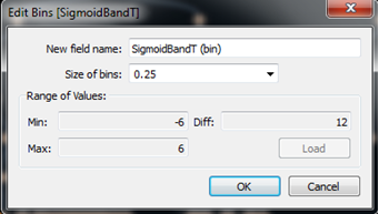
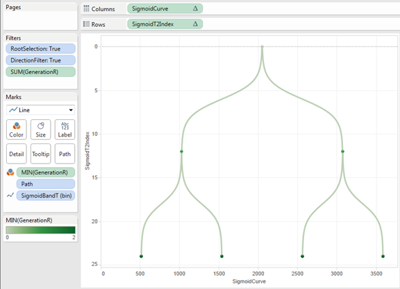
Onto the curves we go. First thing we need to do is add a bin field to generate the path of the curves. We have a field (SigmoidBandT) that is -6 for starting point and 6 for ending point of a node relationship. We bin this field by 0.25 to densify the data and execute the curve equation (make sure show missing values is selected!).

Family Tree Pic 5

When using data densification, we have to be sure to leverage window aggregates for all of the relevant coordinate fields which are needed to drive curve calculations. The start/end points for X and Y coordinates are shown below. One key note is to leverage the FIRST() and LAST() functions to make sure you are only referring to either the start or end point of your paths respectively.

Family Tree Pic 6

Now that we have our bin and windowed coordinates we can build our curves from our parent to child nodes. This is done with two equations (which I found in Shaffer’s node-link tree diagram) shown below, Sigmoid Curve and SigmoidT2Index. One other key field in the formulas is Sigmoid Function, this actually does the math behind the x-value of the curve. (Refer to the work book for the additional calculated fields nested within these formulas.)

Family Tree Pic 7

We replace the rows and columns shelf with the fields mentioned above and place the bin (showing missing values) and path fields on the detail shelf, and we now have curves.

Family Tree Pic 8

One very useful thing that I got from Shaffer’s post was how to do the dual axis when using curved lines. He created a field call Points which is a table calculation that only has a value on the first or last value of a group. I did have to add Node to the detail shelf for Points to work correctly, here is the equation and the updated tree result (now looking a lot like a red-black tree).

Family Tree Pic 9

One last requirement we need to meet is the ability to drill through on any node in the view and see the ancestor or descendant tree from that specific node’s perspective. Here we will leverage the URL action “hack” that Nelson Davis recently blogged about here. Take a look at the details he posted to get a great overview of how this process works and the various pieces of the URL string required for this to work. In addition to this, the other step I had to take was to “cache” the data for the ancestor/descendant tree views having each node as the root. This data preparation work was done in SQL Server in this example and is only required since Tableau Public has limited data connections allowed and data extracts required. You can take advantage of live connections to get around this additional caching step and generate the tree on the fly within your data connection configuration.

So I added two dashboard actions, one for ancestor and one for descendant which use the above mentioned URL trick to hack “dynamic” parameters driving the root node and direction of the tree view. This sends the selected node to our root node parameter and also sends the direction to our direction parameter. Here is an example of the URL action string, I have highlighted the root node and direction parts in green below …

https://public.tableau.com/views/FamilyTree/FamilyTree?:showVizHome=no&:embed=y&:tabs=no&:linktarget=_self&RootNode=<NODE>&DirectionParm=Ancestor

Here is what the URL action menu looks like within the viz…

Family Tree Pic 10

Now, when working on public, we can select any node in the viz and then reset the tree view to either the ancestor or descendant view. Here is the result of selecting ancestor and then descendant views for my grandma on my dad’s side…

Family Tree Pic 11

There are bits and pieces that I have left out of this post to try and keep it from getting too long (still totally failed at that goal). These can all be reverse engineered from the workbook provided or free feel to ping me at @demartsc with any questions. 

Mom – I hope you find this helpful!

Comb the Hairball with BioFabric in Tableau by Chris DeMartini

Screen-Shot-2015-05-09-at-9.43.24-PM.png

Yet another amazing guest post by Chris DeMartini showing amazing options for visualizing for network graph data in Tableau.  I am particularly fond of this one and already have users chopping at the bit to visualize their data this way.  Thank you Chris!

Recently I posted about creating circular and hive plot network diagrams using Tableau and a question was posted around whether we could also execute the BioFabric network graph within Tableau. There is a lot of additional information about the BioFabric network graph at their website. The super-quick demo is a good intro to the graph if you have not seen it before.

The answer to the question posted is yes and this post is designed to walk you through the steps needed to build your own BioFabric graph within Tableau.

First things first the data. I used the same underlying data structure that supported the hive plot network post mentioned earlier. However if you want to save a click, here is a screen shot of what that data looks like. Screen Shot 2015-05-12 at 10.34.45 PM

I also obtained network data generated from Les Miserables, and reformatted the data to match the above structure. Here are the main aspects of the underlying source data requirements: Each edge (relationship between nodes) should have 2 records representing the output node and input node of the edge. Nodes have been numbered based on their degree of adjacency, ordered from highest degree node to lowest degree node. For example node 1 has the most edges, node 2 the second most, etc. My ID field is a combination of the edge output and input nodes separated by a period (e.g. AM.GP is the ID for the edge between nodes AM and GP). This is the identifier for an edge. I also added relationship count which is the number of instances that this specific edge exists in the network.

The above captures the main concepts of the underlying source data, but do review the data within the viz if you want further details.

Onward we go to BioFabric! According to their site (see Significant Features section) I noted the following: Edges are represented as one-dimensional vertical line segments, one per column, terminating at the two rows associated with the endpoint nodes. Nodes are represented as one-dimensional horizontal line segments, one per row. Edges are drawn darker than nodes; this has the effect of emphasizing the links and making them appear to float in front of the nodes. Edges are unambiguously represented and never overlap. Note: There are several other meaningful points in this section of their site, however I am going to focus this post on the ones described above.

Where do we start? Let’s get going with getting edges to show up as vertical line segments.

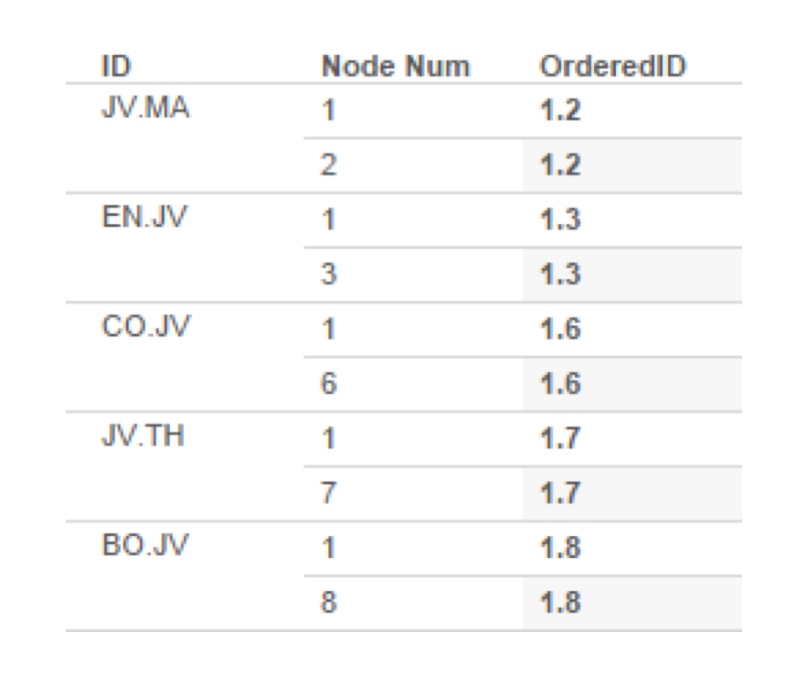
We need a calculated field which I named “OrderedID.” This field was created to address the placement of edge line segments on the X axis. The thought here is to ensure that edges are ordered and grouped based on the degree of their nodes. We want the edges ordered by node degree as follows: edge 1.2 should be before 1.3 which is before 1.10 which is before 2.3 which is before 5.2 and so on. I used the following table calculation. Screen Shot 2015-05-12 at 10.34.53 PM

Which results in this value for the OrderedID field (regardless of edge direction this will place the higher degree node first and the lesser degree node second, assuming node number is ordered). You can play around with this equation (and node number) to modify the placement of your edge segments on your viz. Screen Shot 2015-05-12 at 10.35.07 PM

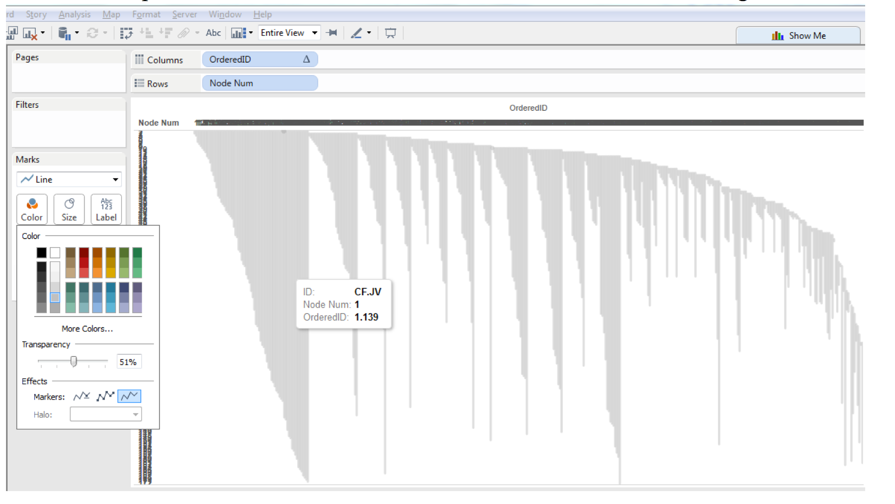
So now we need the Y axis for our vertical lines, this is simply going to be node number. So we drag OrderedID to Columns, Node Number (a dimension in my data) to Rows and make sure that ID is placed on the Detail shelf. Screen Shot 2015-05-12 at 10.35.12 PM

Then we change mark type to line, change view to “Entire View”, change color to gray and 50% transparent and remove markers from lines and we have vertical edge lines! Screen Shot 2015-05-12 at 10.35.18 PM

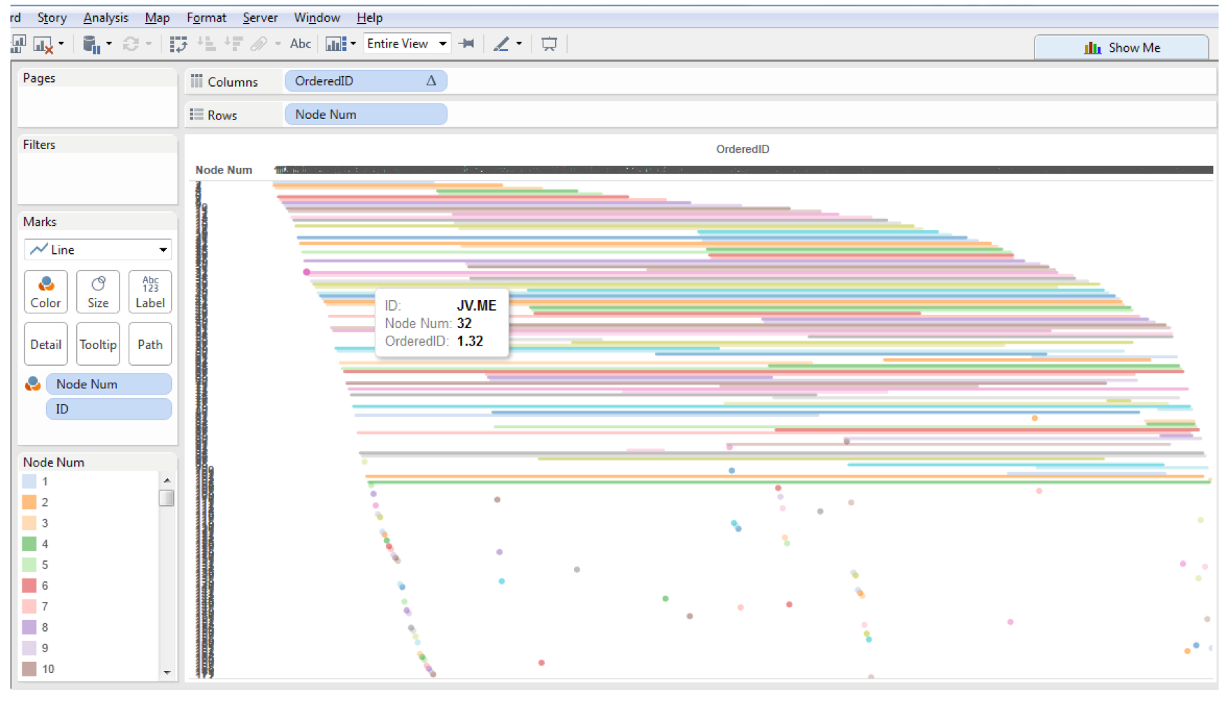
Next we need to get the horizontal node lines and color by node. I first did this on a separate sheet by making a copy of the above sheet. On that copy we then drag node number onto the color shelf and we now see the below. Screen Shot 2015-05-12 at 10.35.22 PM

Sweet! We have one sheet with vertical edge line segments and one sheet with horizontal node line segments, now let’s just put them together right?

One issue you will run into at this point is that Node Number is a discrete dimension, we need to do a dual axis and in order to make that happen we need to convert Node Number to a continuous dimension, after making that change and executing and synchronizing the dual axis we see this… Screen Shot 2015-05-12 at 10.35.28 PM

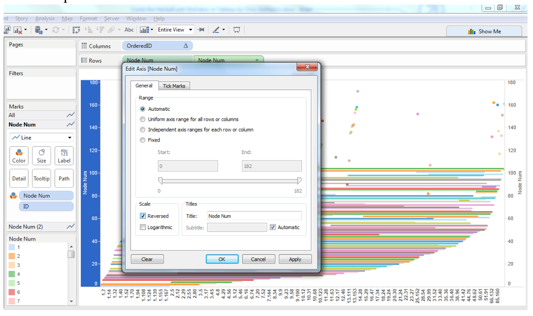
Looks OK, except it is upside down. To fix that we just edit the axis and click the reversed option box. Screen Shot 2015-05-12 at 10.35.33 PM

Now we are right side up again and we need to make a few last changes to combine the two sheets into one view. Here are the steps I took… On the second Y Axis (vertical edges) Drag Node Number from Color to Path Adjust gray color darker or lighter as desired, I used 75% transparency Make sure line size is as small as possible Make sure the second Y axis is in front of the first Y axis Make sure line markers are off Adjust tooltip to you requirements (note: dimensions need to be brought in as attributes to keep from effecting the line paths and table calculations) On the first Y Axis (horizontal nodes) Make sure line size is as small as possible Make sure line markers are on for all points Adjust color transparency as desired, I used 60% Adjust tooltip to your requirements (same rules apply)

Once you have adjusted the Y axes as you want, you can then hide all of your headers from all of your axes, and now we have a BioFabric! Screen Shot 2015-05-12 at 10.35.38 PM

At this point, you can play around with colors, ordering of nodes, grouping of nodes etc. to change the look and feel of the graph. There are some other rulesets which I did not focus on listed at biofabric.org and with some additional work we could probably incorporate those as well.

Hope you find the post and graph type useful, and thanks again for sharing your blog Anya!

Sources: Biofabric.org (graph type source and explanation) https://github.com/mmlc/lesmiserables-character-network (les miserables data)

Building a Visualization of Transit System Data Using GTFS

Screen-Shot-2015-05-02-at-4.56.10-PM.png

Yes, yet another Allan Walker and Anya post about mapping things :-).  This one however is a precursor to some very fun JS API how to's, including how to animate the viz, coming soon featuring Chris DeMartini .  Stay tuned!

Q:  Um, what is GTFS? 

A:  The General Transit Feed Specification (GTFS) defines a common format for public transportation schedules and associated geographic information. GTFS "feeds" allow public transit agencies to publish their transit data and developers to write applications that consume that data in an interoperable way.

https://developers.google.com/transit/gtfs/ 

Screen Shot 2015-05-02 at 4.51.10 PM

Q:  And I care because? 

A:  Use Tableau to build a map of transit data and incorporate it in a BI dashboard for analysis.  What is the average route duration, fare, number of stops?  How many are wheelchair accessible?   Don’t care about BART?  Check out the list of all the agencies that use this format at http://www.gtfs-data-exchange.com/agencies .

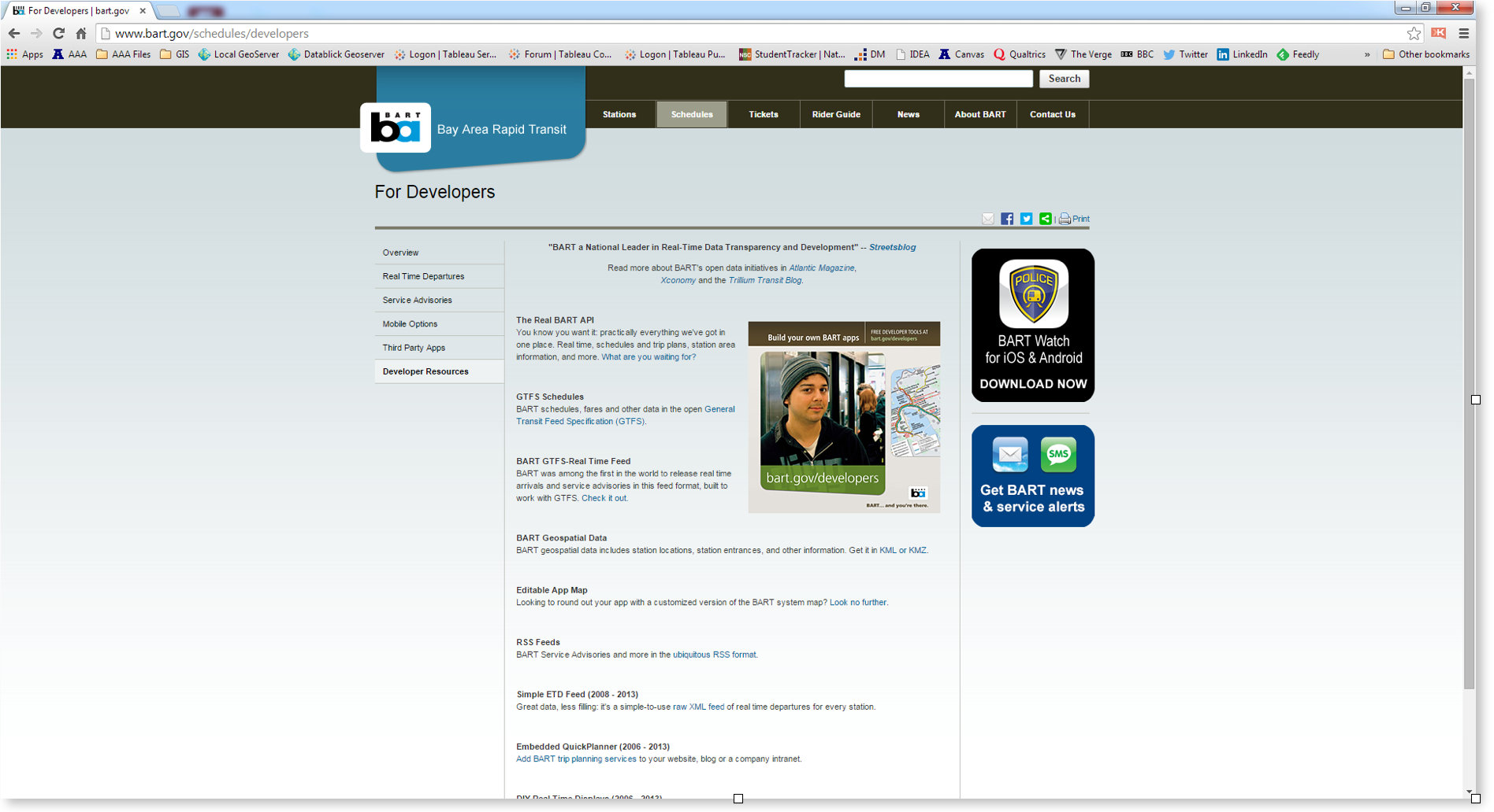
Step 1:  For the sake of this demo, visit the http://www.bart.gov/schedules/developers

Screen Shot 2015-05-02 at 4.51.02 PM

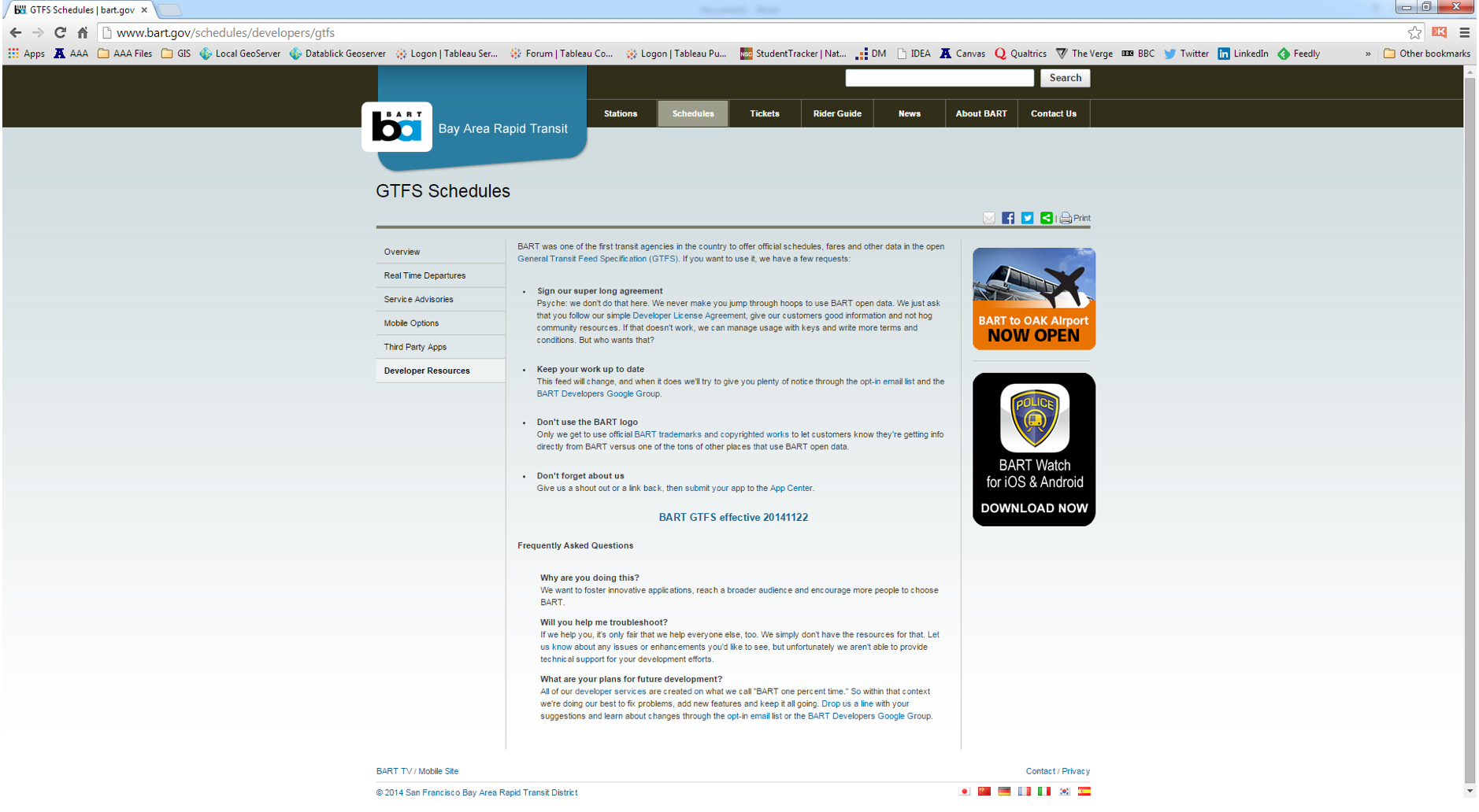
Step 2:  Download the GTFS zip file at http://www.bart.gov/schedules/developers/gtfs

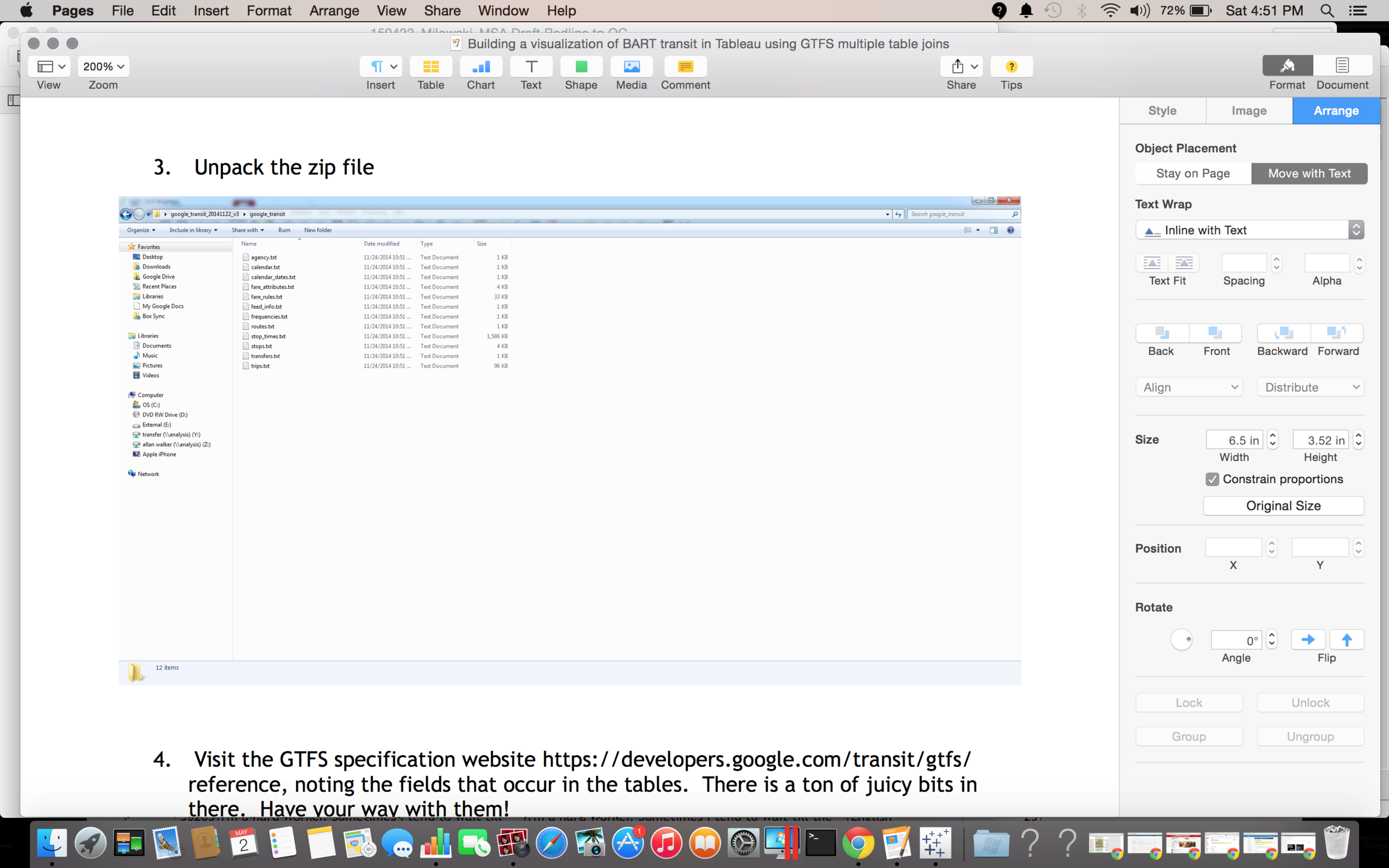
Unpack the zip file

Screen Shot 2015-05-02 at 4.51.14 PM

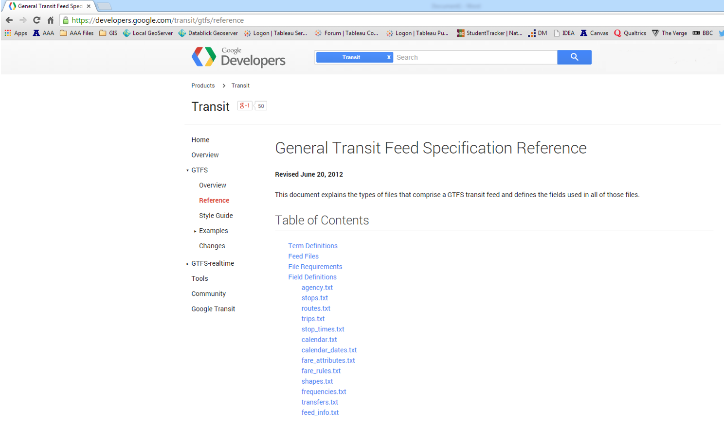
Visit the GTFS specification website https://developers.google.com/transit/gtfs/reference, noting the fields that occur in the tables.  There is a ton of juicy bits in there.  Have your way with them!

Screen Shot 2015-05-02 at 4.51.18 PM

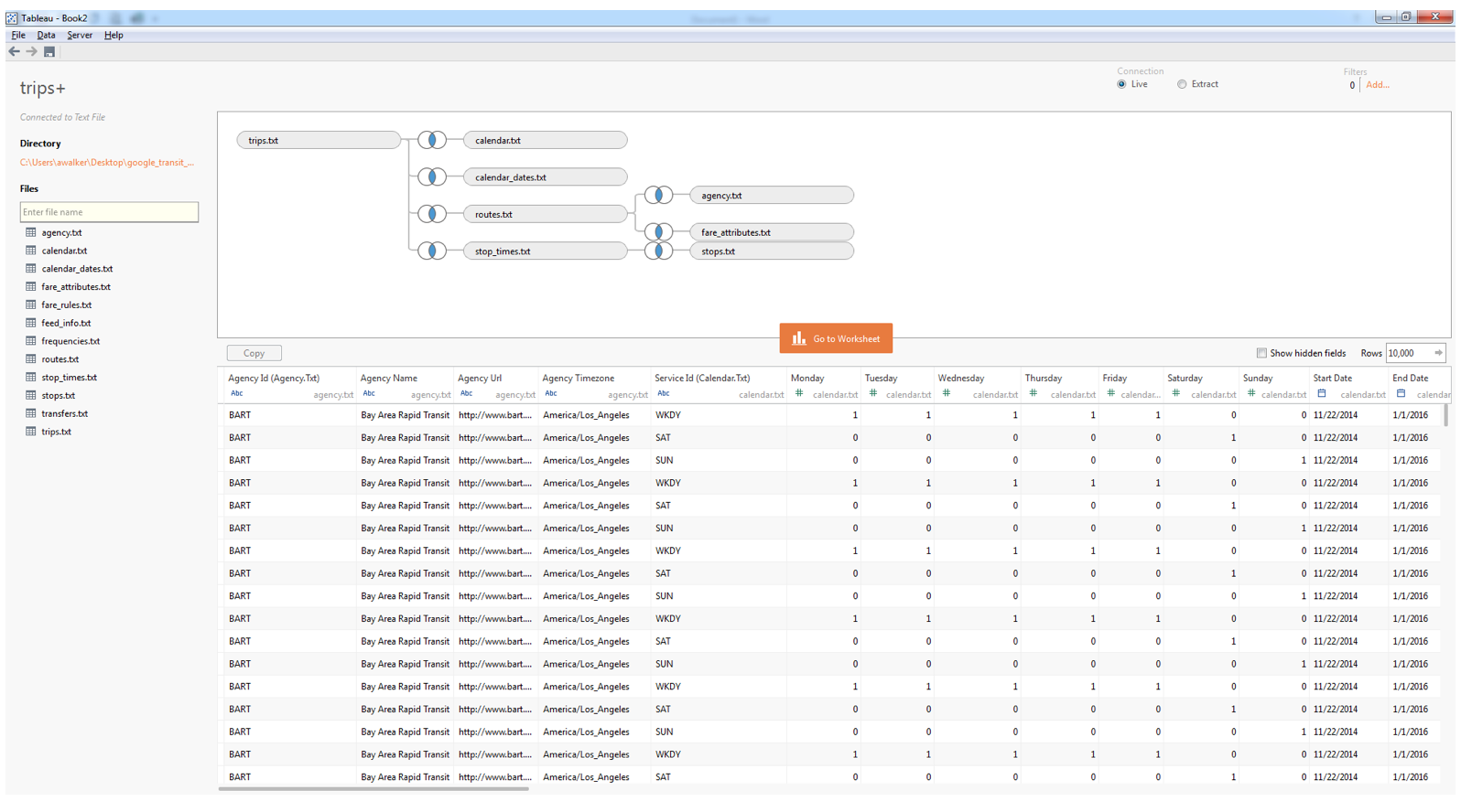
Fire up Tableau and begin joining the tables.

Start with the trips.txt

The joins are inner and magically delicious and just happened when you click a table to add it, but just in case here they are:

  • trips.txt to calendar.txt on service_id
  • trips.txt to calendar_dates.txt on service_id
  • trips.txt to routes.txt on route_id
  • routes.txt to agency.txt on agency_id
  • routes.txt to fare_attributes.txt on agency_id
  • trips.txt to stop_times.txt on trip_id
  • stop_times.txt to stops.txt on stop_id
  • Extract the data (Optional – filter for a specific day to speed things up a bit while you play with the data)

Screen Shot 2015-05-02 at 4.53.41 PM

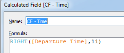
Let’s create our first Calculated Field (CF), based on [Departure Time]:  “CF-Time”.  First, change [Departure Time] to a string, and add the calculation:

RIGHT([Departure Time],11)

Screen Shot 2015-05-02 at 4.53.48 PM

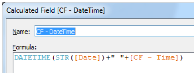
Next, let’s create another Calculated Field to concatenate [Date] and our [CF -Time] field: “CF-DateTime”.

Screen Shot 2015-05-02 at 4.54.11 PM

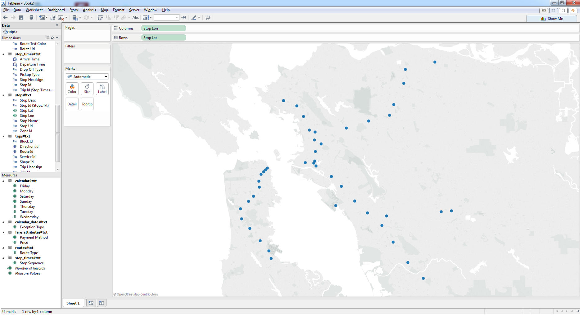
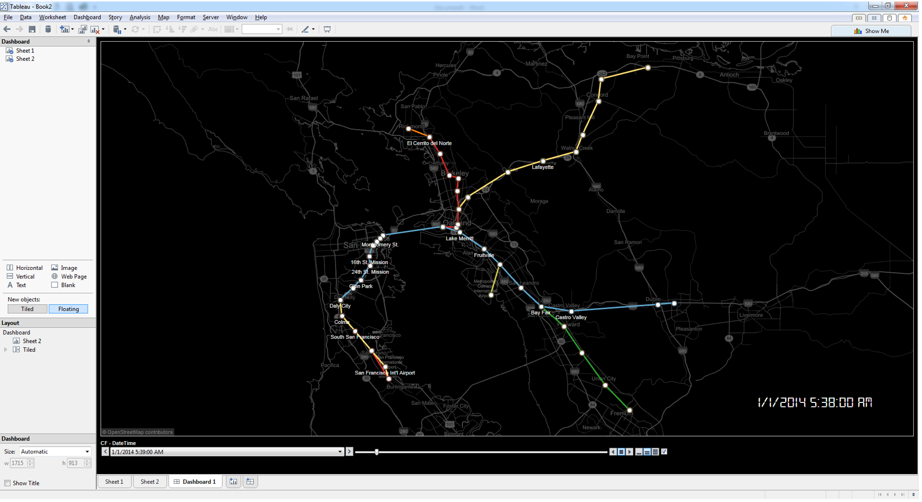
Make sure that your [Stop Lat] and [Stop Lon] are dimensions.  Drag [Stop Lon] onto the columns and [Stop Lat] onto the rows.  You can now see all the stops (BART Stations) on the BART route.

Screen Shot 2015-05-02 at 4.54.34 PM

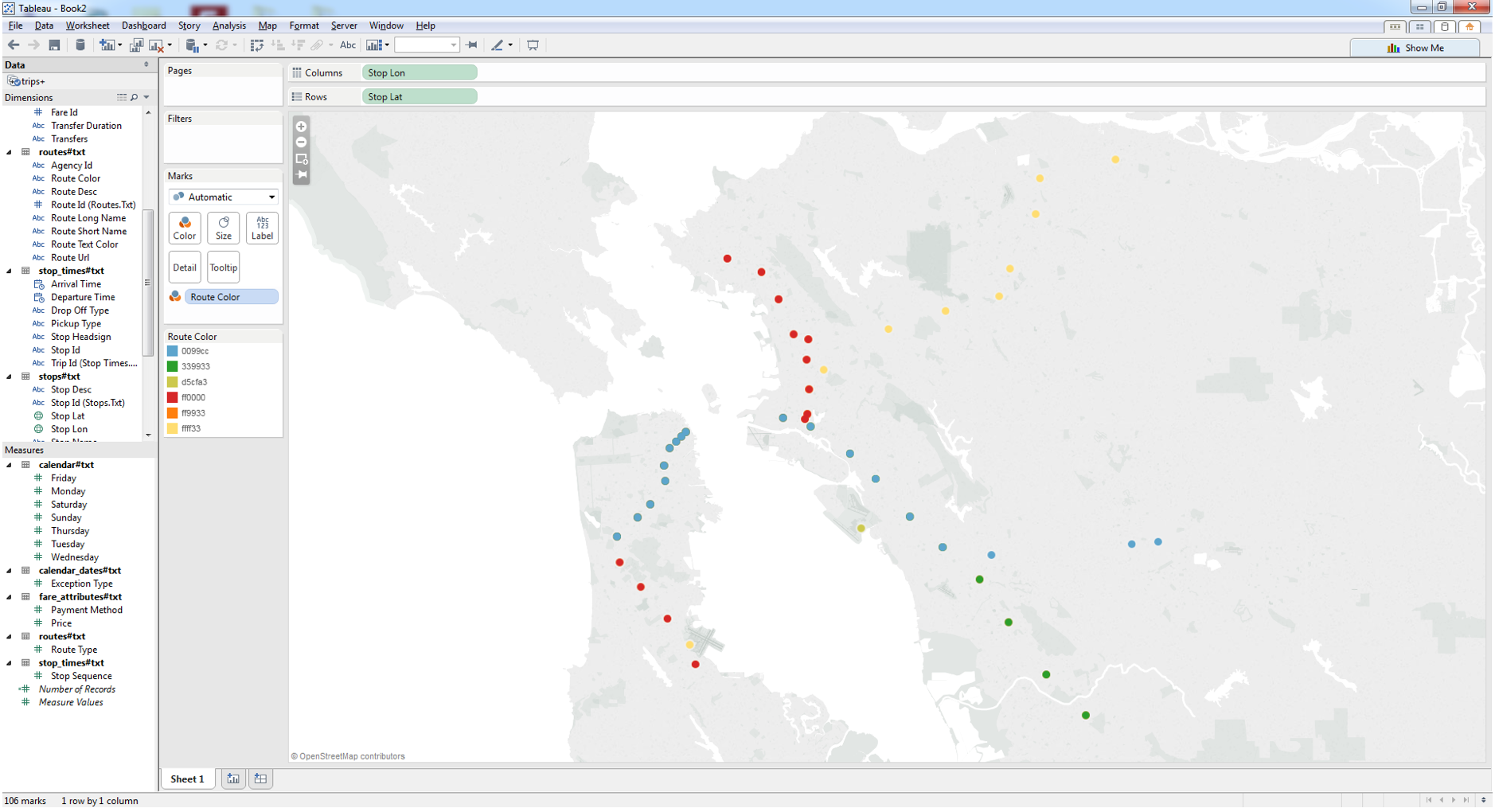
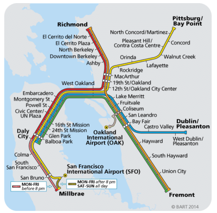
Drag [Route Color] onto color – these are hex values that correspond to the color of the BART system map.  (Note that some stops are serviced by more than one route, and only the top color in the sort order will appear. 

Screen Shot 2015-05-02 at 4.54.43 PM

You could go pie chart on the stops, but you would be harassed to no end by Andy Kriebel.   If you need to convert Hex colors to RGB, use a website such as http://hex.colorrrs.com/, otherwise change the colors in Tableau to match the Hex code.  They will now match the colors on the real BART Map.

Screen Shot 2015-05-02 at 4.53.53 PM

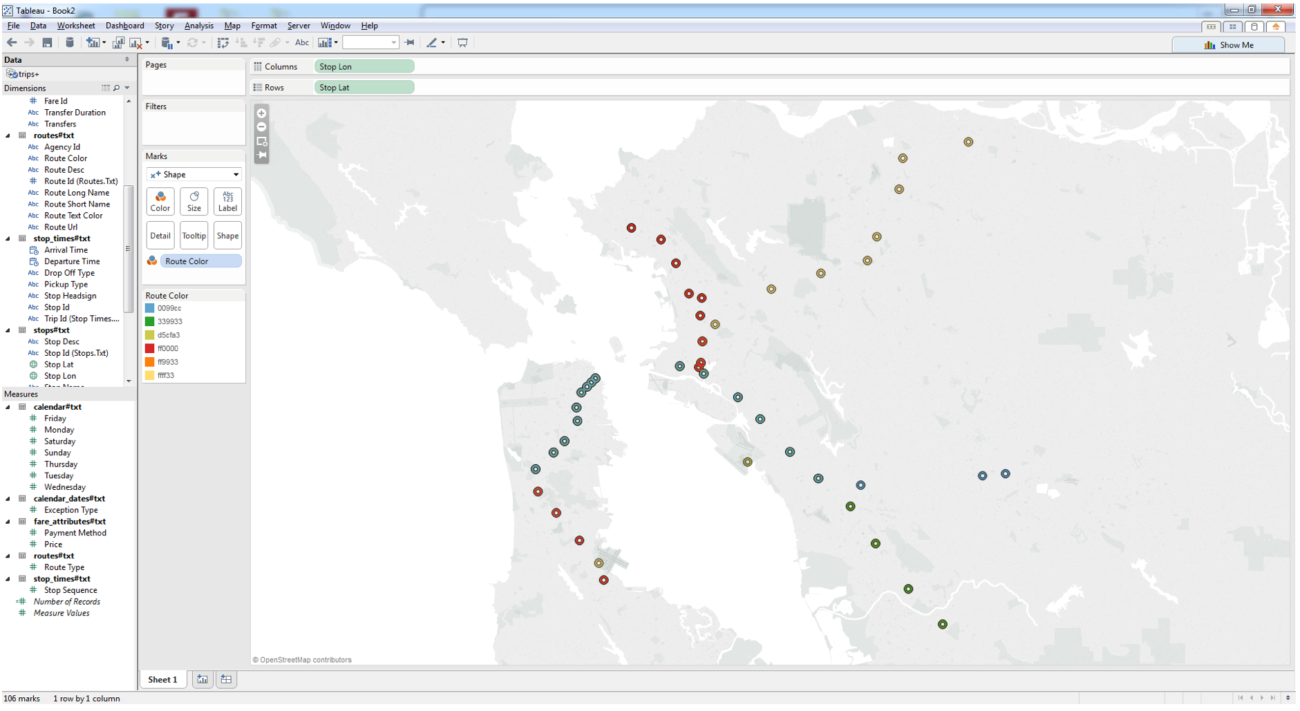
Make sure the mark shape is a filled circle and add a black halo using the color card.  This is just for formatting but it will make the stops look more like the ones on the original BART map when you are done.

Screen Shot 2015-05-02 at 4.54.48 PM

Then Move the [CF – DateTime]  to the Pages Shelf.  Using the arrow to the right of it, choose Exact Date.  This will speed things up, but also let you see what a day in the life of the BART looks like.

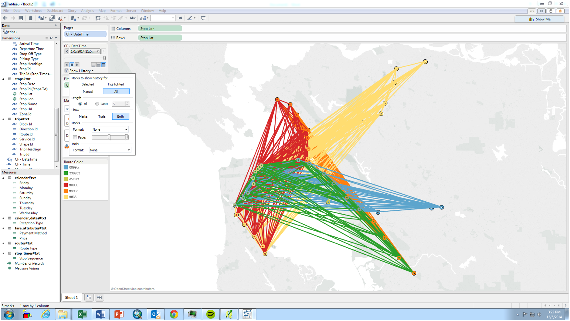
Check the Show History box, selecting “All” history and “Both” marks and trails. 

Screen Shot 2015-05-02 at 4.55.01 PM

Drag the Pages slider all the way to the right or just hit play and wait (or go get a beer while it plays).  It's a total mess!

Screen Shot 2015-05-02 at 4.55.14 PM

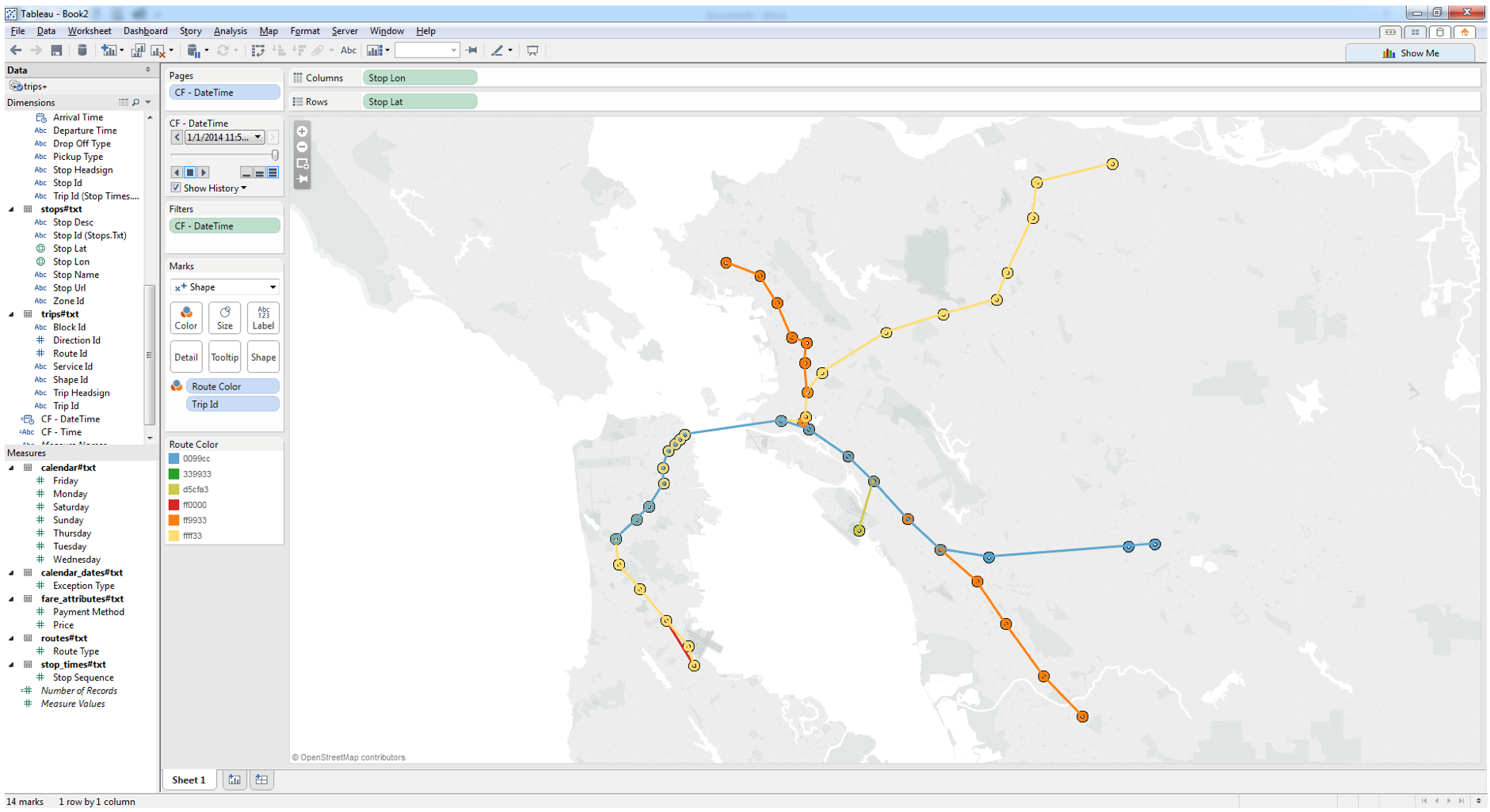
Drag [Trip ID] onto Level of Detail

Click “play” on the slider to see trains depart each station on the BART Routes!

Screen Shot 2015-05-02 at 4.55.18 PM

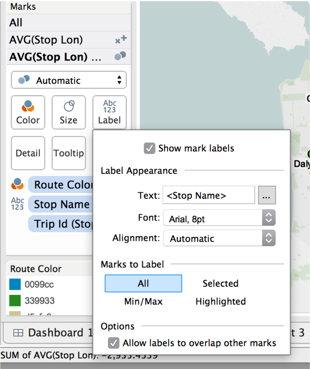
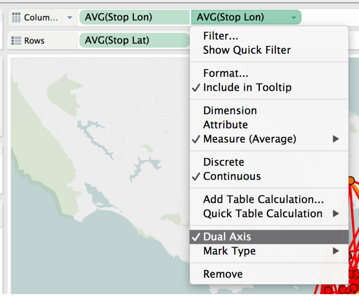
Let’s add some labels, and tidy up the stations.  Add [Stop Lon] again to the Columns Shelf and create a dual-axis. 

Screen Shot 2015-05-02 at 4.55.22 PM

Change the mark type to circle for the second mark type.  Remove the Color pill for [Route] and change the color of the circles to white if you want to look like the example.  Add [Stop Name] to Label, allowing labels to overlap other marks

Make the Map Black, because Allan likes to get all Johnny Cash and makes everything a black.  But really, just go to your Map menu, and select Map Options and play to your hearts content. 

Screen Shot 2015-05-02 at 4.55.29 PM

Now it’s time to create a dashboard with our map.  Add the map you just created to the dashboard and move the pages controls to the bottom.

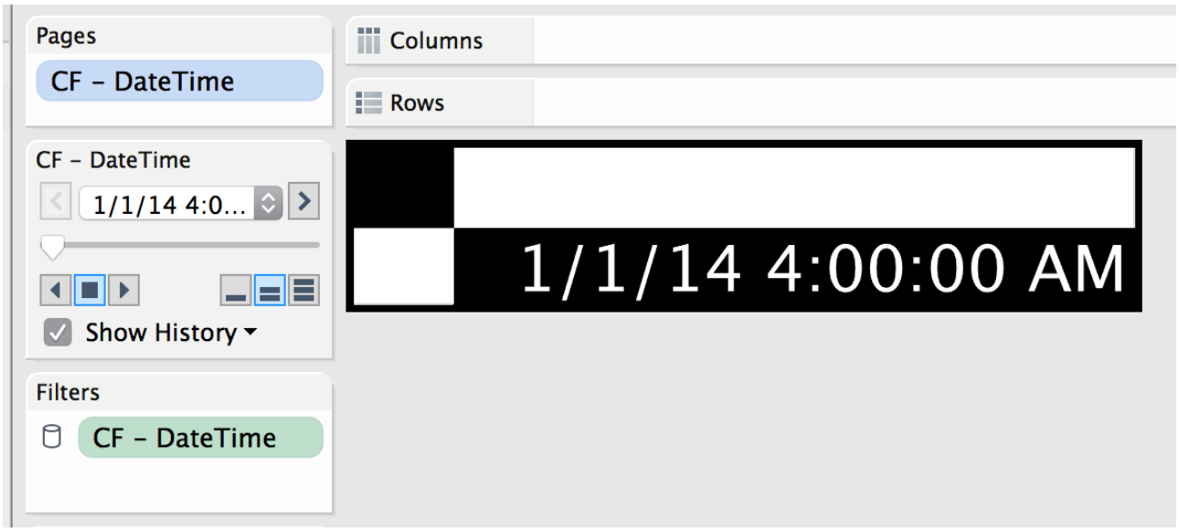
Let’s create a “timer” in a second worksheet.  This will display the latest time being show in the Pages Shelf.  In the new worksheet, Drag [CF-DateTime] to the Pages area and change to show Exact Date just like we did on the other worksheet.  In “Show History”, only show the last 1 mark, also check the “Fade” box. 

Add [CF-DateTime] to the Text card, and change it to Exact Date.

Screen Shot 2015-05-02 at 4.55.31 PM

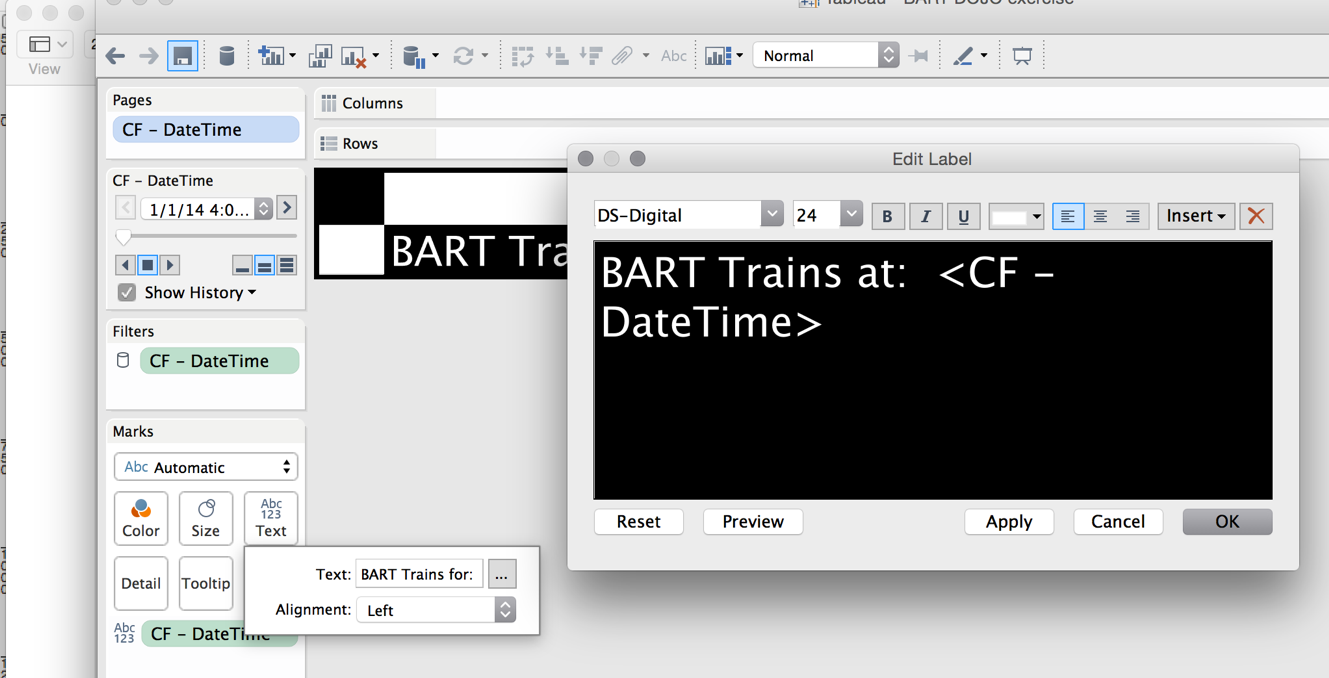
We will use this sheet as the header of the dashboard.  Click on the Text Card and add the text “BART Trains at: “ before the field [CF-Datetime]  Make the text big, and bold and in the color of your choice. 

Screen Shot 2015-05-02 at 4.55.34 PM

Add Sheet 2 to your dashboard at the top and hide the title.

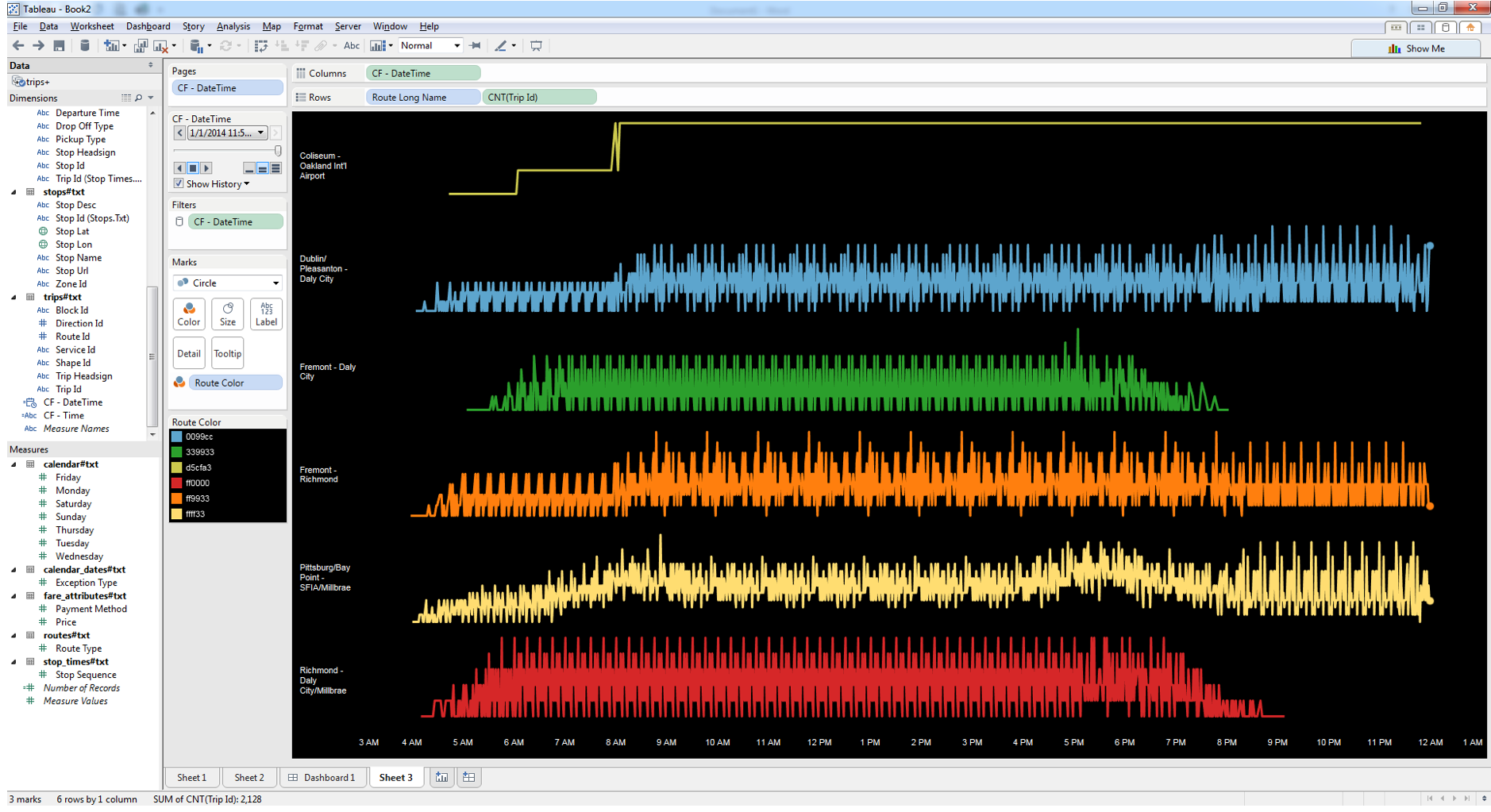
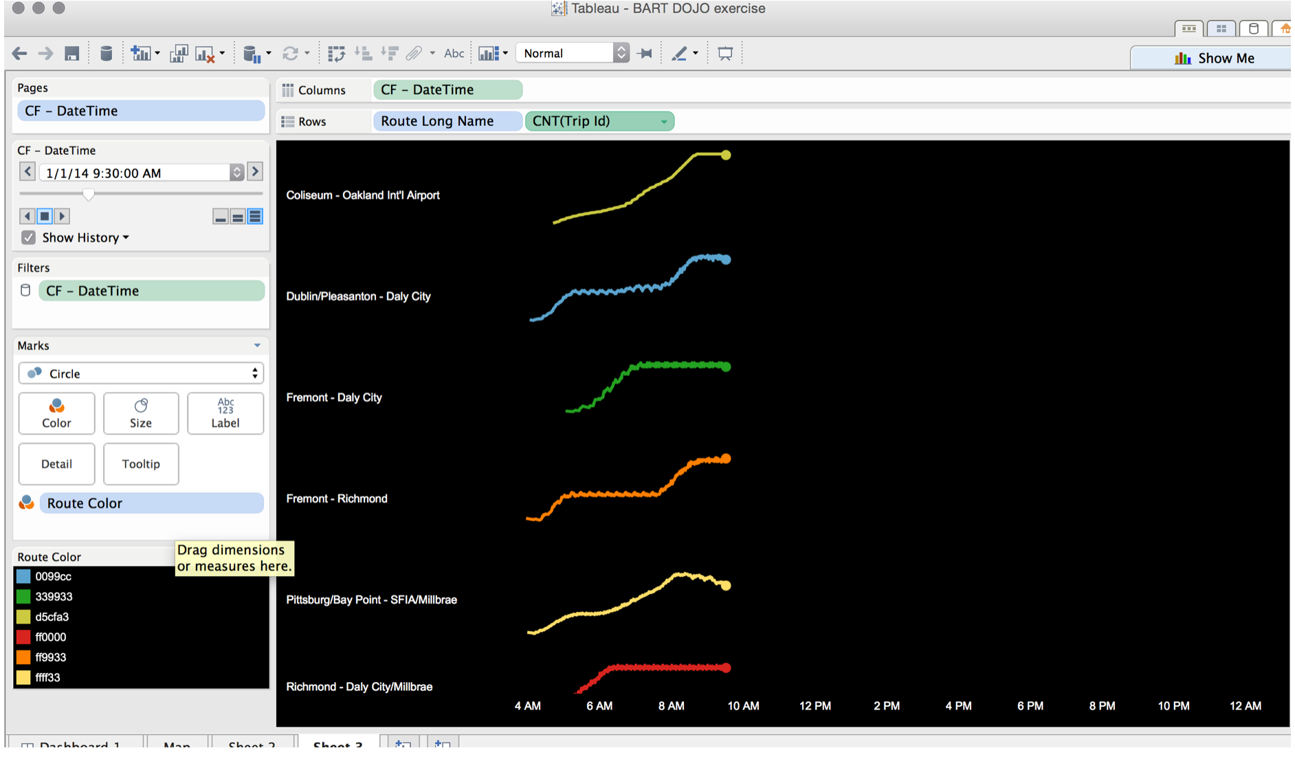
Let’s build some charts to complement the map.  Sheet 3 is built using the set-up of circle mark type, history as trails,  and a Count of the TripID by Route Long Name in the Rows:

Screen Shot 2015-05-02 at 4.55.47 PM

The view above shows for each minute or two that the pages go through how many BART trains actually have a record.  As the trains only have a record when they depart a station and it may take more than a minute or two to reach the next station, you may choose to create moving average of the count of the [Trip ID] to smooth out the lines a bit.

Screen Shot 2015-05-02 at 4.55.39 PM

Add any new views to the dashboard, but remember for the animation on the Pages slider to work, they all need to have the [CF-DateTime] in the Pages shelf, and all need to be set to “Exact Time”.  Rearrange, and bend to your will.  Go get another beer and show a friend how much you rock now that you can animate transit systems in Tableau, and mix BI, Data Viz and GIS together.

Screen Shot 2015-05-02 at 4.56.10 PM

Optional Note:

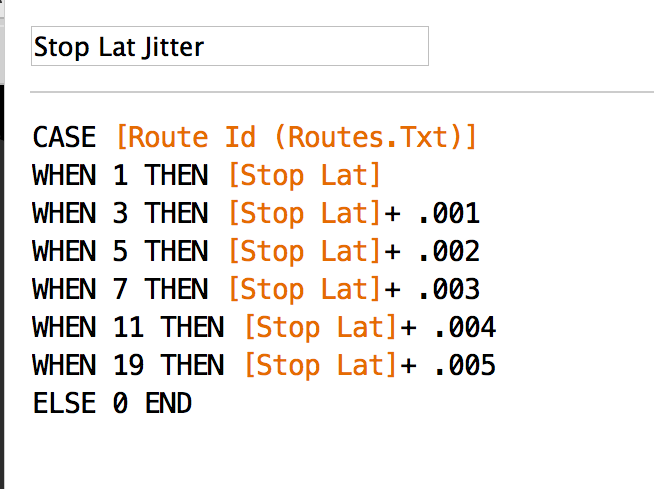
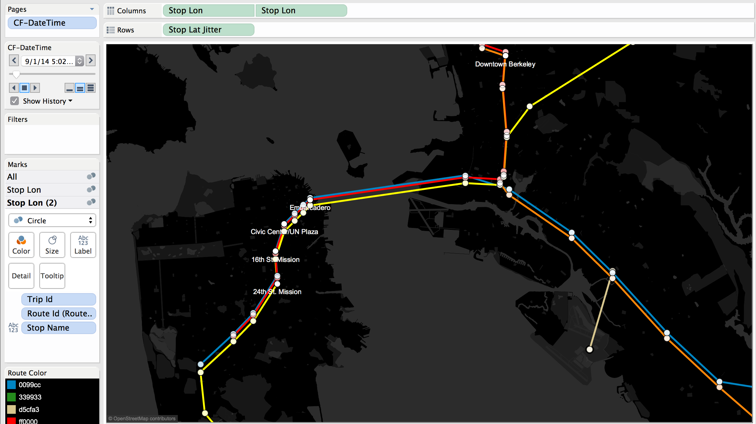
Perhaps the fact that the lines overlap bothers you, as only the top line shows.  If so, just add a bit of "jitter" to your lines to space them a bit apart.

Screen Shot 2015-05-04 at 2.24.14 PM

Screen Shot 2015-05-04 at 5.11.13 PM

Give that Tableau Workbook a Makeover with "Find and Replace Gone Wild!"

Screen-Shot-2015-04-12-at-8.28.38-PM.png

I had the distinct pleasure of presenting at the Tableau Think Data Thursday today along with Kelly Martin and KK Molugu.  There is a whole library of awesome, so forget Daredevil and spend a night watching all of those, or open a bottle of wine and get jiggy with me and your .twb. Okay girlfriend, I know you said you didn't code, but hey, let's go there.  It'll be fun. I promise, and no one will be able to tell if she did or didn't.

So here is the use case.  Lets say your corporate font just got changed from Arial to Segoe UI.  Or, you are just plain tired of having to format your Quick Filters, turn on and off your those pesky tooltip buttons, or want all your field labels to always be hot pink with glitter.  I am still waiting for the glitter feature in Tableau by the way.... hint hint.  You could spend a day changing  your workbooks, yawn!  If you are lucky you have a corporate Sugar Daddy who will buy you Power Tools, an amazing product, do that.  But if not, you can get similar results from DIY Find and Replace in your favorite text editor.  I use Notepad ++ on a PC or Sublime Text on a Mac.

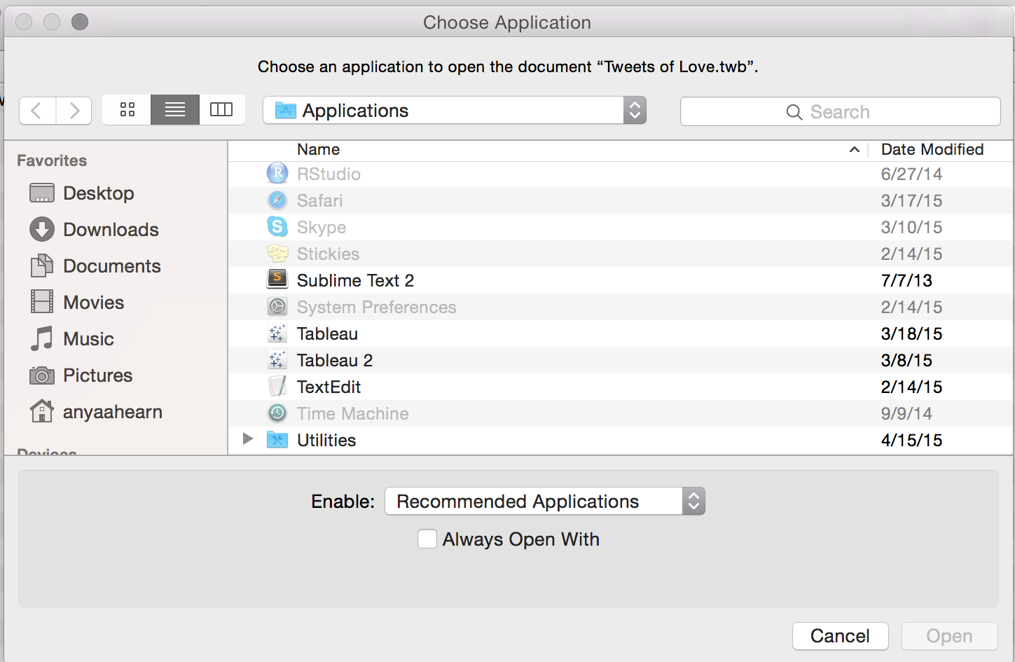
Is your bottle of wine open yet?  Or even better a bottle of Ballast Point Sculpin?  Then go to the workbook in desperate need of a makeover.  Make a copy of it.  This is an un-supported hack so always back up!  Browse to your copy in the Finder window.

Screen Shot 2015-04-23 at 6.29.52 PM

and open it with the text editor of your choice.

Screen Shot 2015-04-23 at 6.30.01 PM

You will now see your workbook for what it really is, a bunch of XML waiting for you to have your way with.  Go ahead, scroll about and see all the fun to be had.  Or, get down to business and start searching for things that may be of interest, like your font.  Using "Find" search for something like

font-family

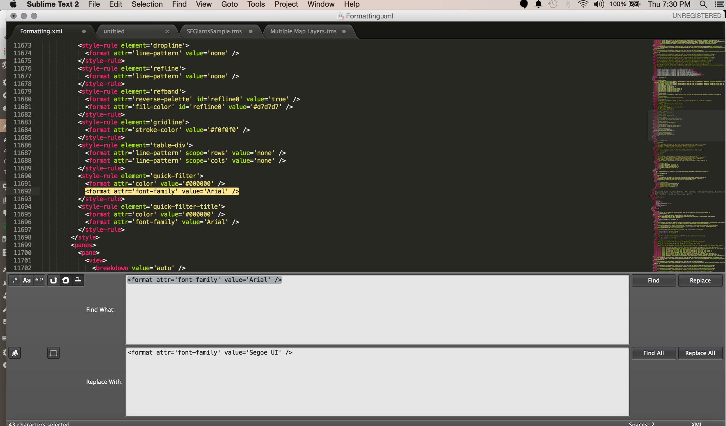
My font was Arial - so last season.  How embarrassing.  <format attr='font-family' value='Arial' />

Screen Shot 2015-04-23 at 7.30.30 PM

This season Segoe UI is the new black so just "Replace" all your <format attr='font-family' value='Arial' /> with <format attr='font-family' value='Segoe UI' />

Save the file and re-open in Tableau and instant makeover!  Did you just feel the rush of power!  Come on.  Do a little more.

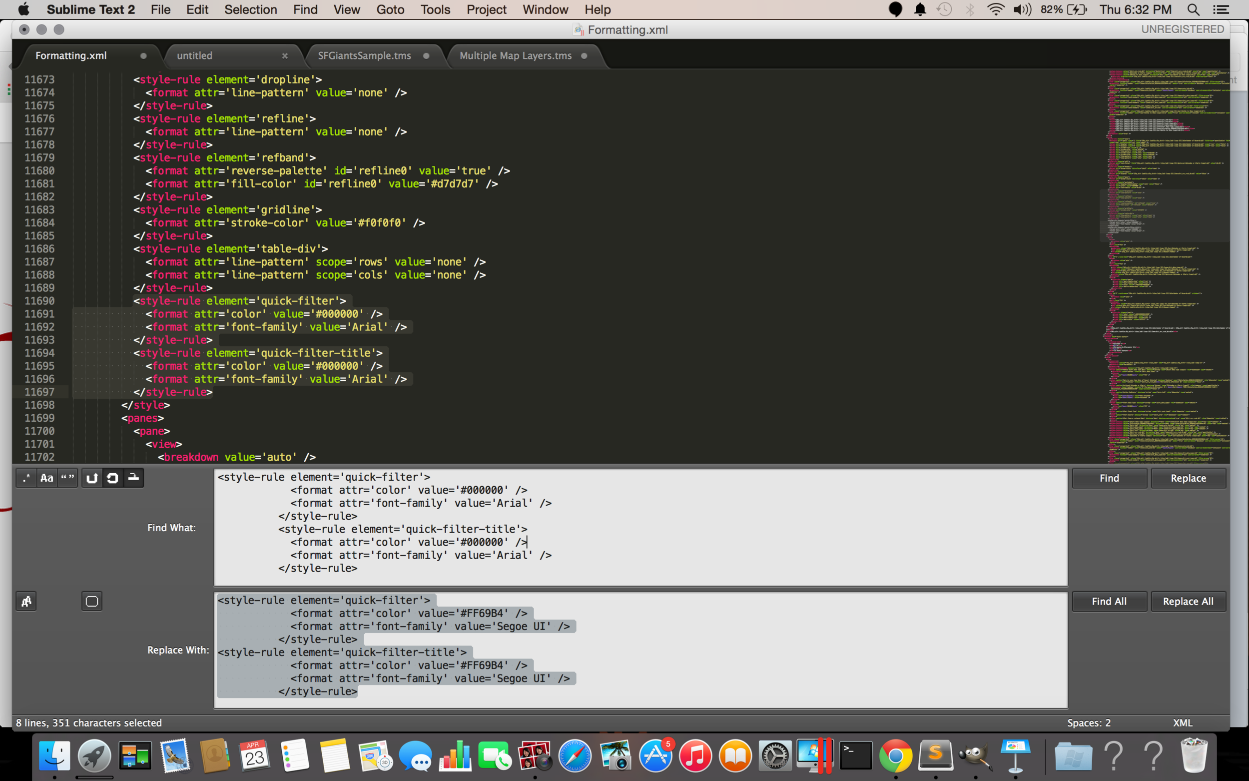
Gussy up your Quick Filters:

<style-rule element='quick-filter'>

            <format attr='color' value='#000000' />

            <format attr='font-family' value='Arial' />

          </style-rule>

<style-rule element='quick-filter-title'>

            <format attr='color' value='#000000' />

            <format attr='font-family' value='Arial' />

          </style-rule>Screen Shot 2015-04-23 at 6.32.57 PM

Or make all your field labels hot pink

<style-rule element='field-labels'>

            <format attr='color' value='#000000' />

            <format attr='font-family' value='Arial' />

          </style-rule>

Or turn of those pesky tooltip buttons

<customized-tooltip show-buttons='false'>

 Anyhow, have at it, have fun, and don't forget to always make a copy, just incase you break something with a typo.  Enjoy!

Create multiple custom map layers in Mapbox that you can toggle on and off in Tableau

MainTwitter.png

Yes, this is another Allan Walker and DataBlick co-production.  It is also based on the work of the amazing and talented Craig Bloodworth who figured out how to incorporate Mapbox in Tableau and graciously gave my first .tms file.  Allan and I worked on many aspects of the project together and this is a joint post with half on DataBlick, focusing on the maps, and the other on his blog, focusing on sentiment analysis and using Voice Control.

If you haven't already, please start with the post http://datablick.com/2015/02/04/fast-and-fabulous-custom-maps-using-mapbox-in-tableau/,

This adds onto the Mapbox customization for Tableau by showing you how to:

  • Import custom shapefiles
  • Edit them in QGIS (optional)
  • Style them in Mapbox
  • Add them to a Tableau .tms so you can toggle them on and off in many combinations to help your visual analysis.

If you want to click along and learn, please download the latest version of Mapbox Studio at mapbox.com  You will need a Mapbox account.  Warning, you will probably want to be able to have multiple maps as this point and might need a paid account which is about 5$ a month.  I find it better than shoe shopping, so I am up to the 50$ a month account.  My new guilty pleasure!

Optional, download QGIS if you want to get fancy with your own shapefiles.

The final viz, “Finding Love on Twitter” was created as an  excuse to showcase how multiple map layers created in Mapbox for use in Tableau, and the ability to toggle them on and off.  It was for a presentation at the SFTUG graciously hosted by Daniel Seisun and the kind folks at Twitter.

We each seem to have a different take on how this project got started.  You can read what "he said", or you can just believe me ;-P.  It shows a fun contrast and collaboration of how we each came into the project and how we egg each other on.

In response to Allan's intro:

Really? That's how it went down?  So don't remember that at all, but I was on my 2nd Manhattan and a few shots of some bizarre moonshine that Noah and Joe had brought.

I recall feeling a bit bitter about the topic of "love".  I wanted to capture the tweets for things that were both about love on Valentines day, and then of course what someone who was anti-Valentines might tweet.  #Love vs #Hate or #Sex (not sure what the “opposite” is), #Champagne vs #Whiskey (or #beer), etc. It would all culminate in a horrific R. Crumb'esc commentary / viz.  I was particularly excited about a Mapbox style called “Pencil” that would be perfect.
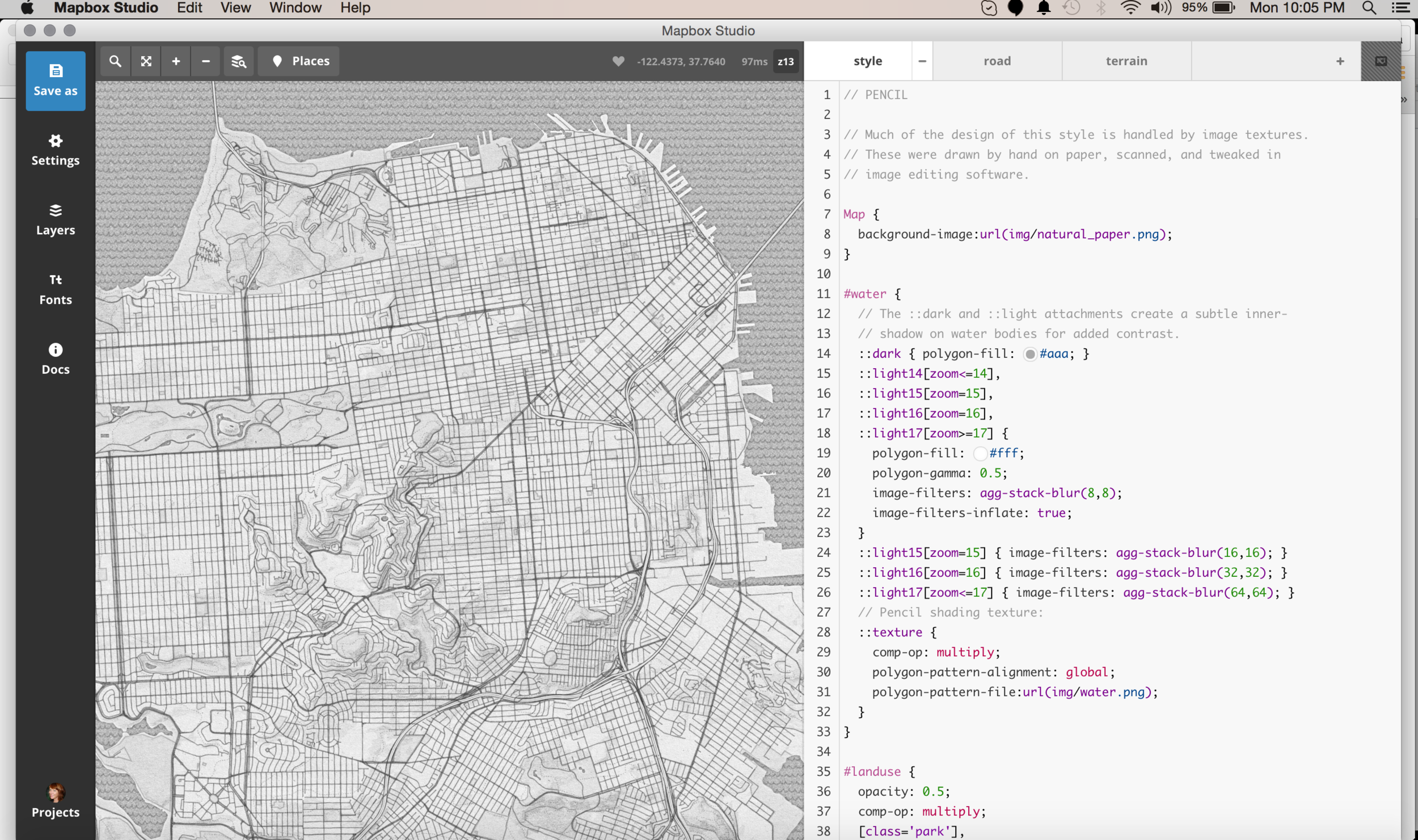
Screen Shot 2015-04-13 at 10.05.05 PM

Smack down data design lesson 1.  Wait for the data to tell the story and determine the design, not the design to determine the story.

As usual, Allan sprang into action, and about 5 whole minutes later had set up pulls of tweets on various hashtags to be archived in google spreadsheet by hashtag.  Set it and forget it, right?

Well some time goes by, and it is actually getting to be close to Valentines day, and so I go to check on the “crock pot” Google sheets that have been supposedly simmering and getting juicy with love tweets, only to find that the volume and content of Geo-tagged tweets is best to be described a “Meh”.   There is no "bitter" to be displayed in all of it’s glory.  There are like 100 tweets and they are all really, really boring.

I am presenting at an upcoming SFTUG at Twitter on creating Mapbox maps for use in Tableau.  If anyone can help get me “tweets of #love”, surely Twitter can!  And graciously they agree to!  Thank you Daniel!  By now though, I am not so bitter, and also am kind of embarrassed to ask for tweets on  things like #sex and #whiskey and decide that maybe just looking at #love would be good.  But of course I want to use a Mapbox map of the world, and the world doesn't only tweet in #love to talk about love.  So of course Allan produces a list of words used for love in the top 20 languages used in the world in under 2 seconds flat, and it is off to the kind folks at Twitter. 

Super excited!  Twitter data from the fire-hose!!!!!!  There “got to be gold in them tweets”!

Sadly no, still “Meh”.  At best we created an Esty’s like cartoon of love raining down by country.  Most of the tweets were actually for free giveaways and contests.
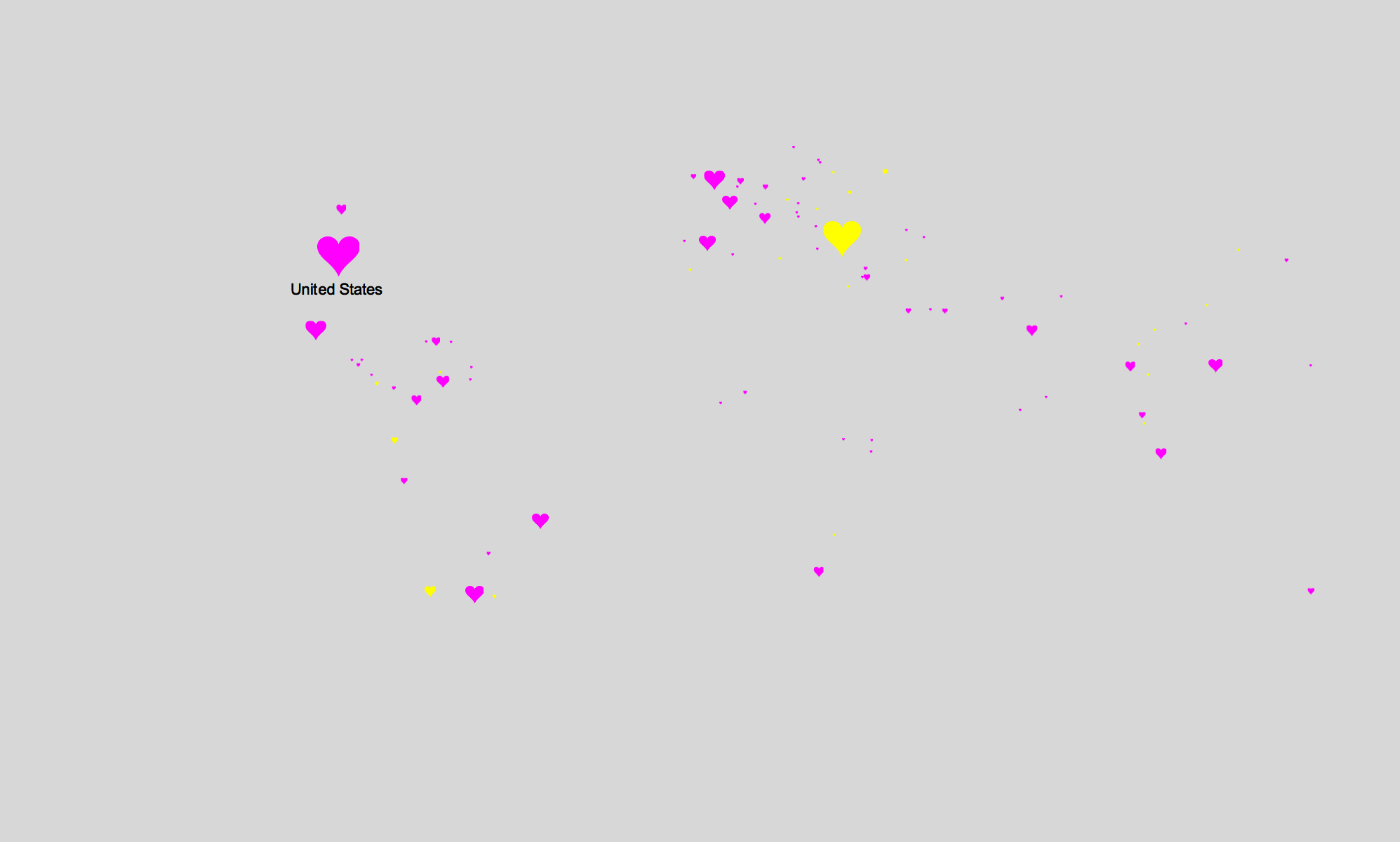
Screen Shot 2015-04-15 at 4.43.57 PM

Exploring all the tweets, the most are for @IntelJapan and @IloveHQ for a giveaway contest.  Super romantic, right?  I did love looking for the haters, since Allan added a bunch of Sentiment Analysis courtesy of Semantria.
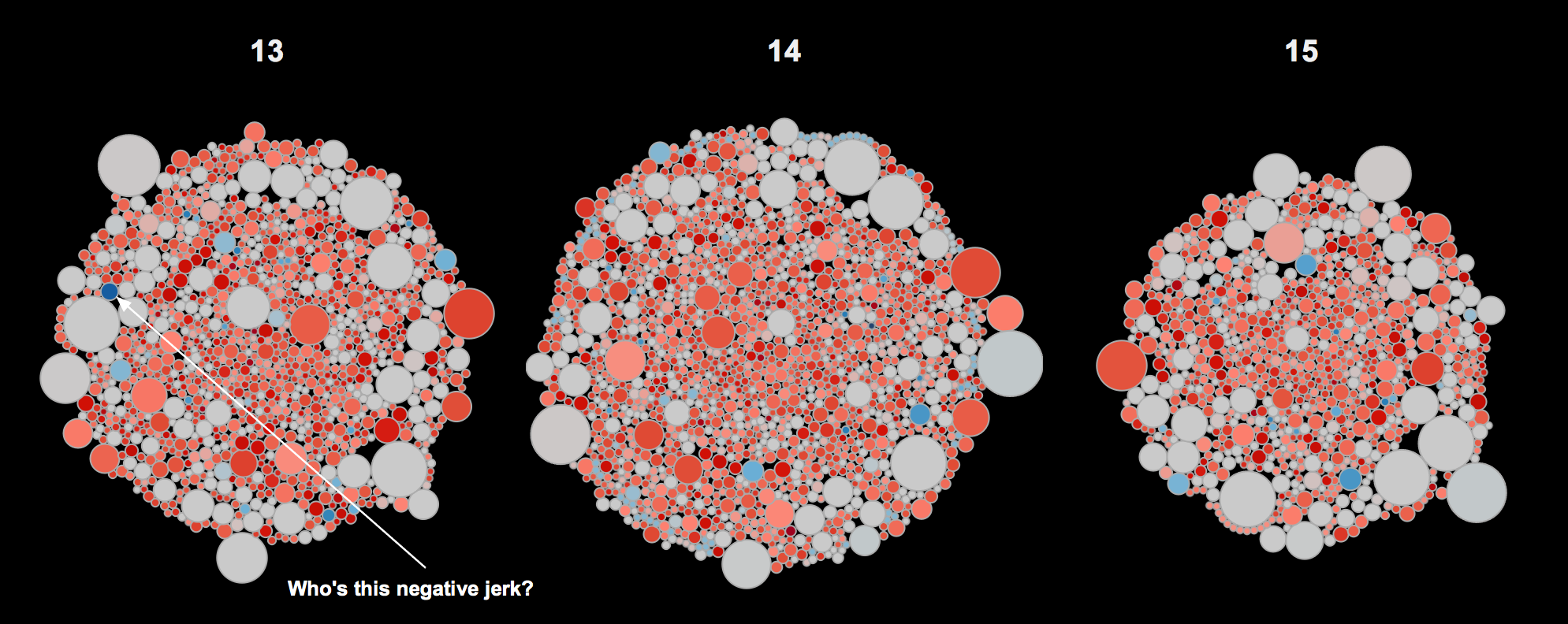
Screen Shot 2015-04-15 at 4.56.08 PM

Well, I still have to present at the SFTUG and I still am committed to making the data about #love on Twitter, so when the data fails you, whip out your design card and put some lipstick on it…  The resulting concept was to use the Twitter data to create an App to help me "Find Love on Twitter".  

Lesson 2, even though you make it pretty, if the data is boring, the viz ain’t gonna sing.

In #love with my new Mapbox skills, I wanted to take them to the next level by being able to not just customize their existing fabulous, out of the box styles, but add my own layers, layer then on top of one another, and be able to turn them on and off in Tableau.  You might want to do something similar to add congressional districts, agricultural land plots, etc.  My example is a bit more silly, but the process is the same.

My design inspiration.  I had just been to the Keith Haring exhibit at the deYoung and really enjoyed this painting:

monster-eats-man

“The TV monster and the helpless man.”   Haring’s figures are captives and victims of forces they may have created but no longer control.  I kind of really liked this messaging and aesthetic applied to a concept of online dating based on social media data and decided to create my “Finding Love on Twitter” viz with a similar aesthetic. 

Now come click along and get to some map making!

Starting with the Mapbox Style “High Contrast”, I set out to create the background map for my #love viz.   If you want more information on custom map styling, using a pre-defined map source in Mapbox, please refer to my previous post at  http://datablick.com/2015/02/04/fast-and-fabulous-custom-maps-using-mapbox-in-tableau/

If I was really going to create a faux viz “app” that I would use to find #love based on Twitter data, I needed to stretch the ridiculous that much more.  I wanted to be able to add other geodata to the mix to show off my new custom Mapbox layers skills, and came up with the idea of being able to turn on and off MUNI railway lines, because I could obviously only look for love if someone lived near public transportation, and also to create shape files of neighborhoods that I would not consider finding love in.  Sorry Marina boys.

A very simplified description of map making is to think that everything for the most part is either a points, lines or shape (polygon), and you style each and then put them all together to make a map.  To style them in Mapbox you use CartoCSS which is very similar to styling a web page.  An example would be:

#layer {

  line-color: red;

  line-width: 2;

}

Where the #layer is the name of a layer, for example streets, and the style of the lines in that street layer are a red line with a width of 2 pixels.

Let’s go find some shapefiles layers to import. 

Thankfully there are many free shapefiles out there to take advantage of, such as a google search showing a ton of shapeless for San Francisco.  I usually use this site: https://data.sfgov.org/data?search=shapefiles&dept=&category=&type=

Your downloaded files will most likely be in a folder that contains 5 files.  These files have the same name, but different extensions.  You will need them all, and they need to be zipped in one file to import to Mapbox.

Optional QGIS Step:

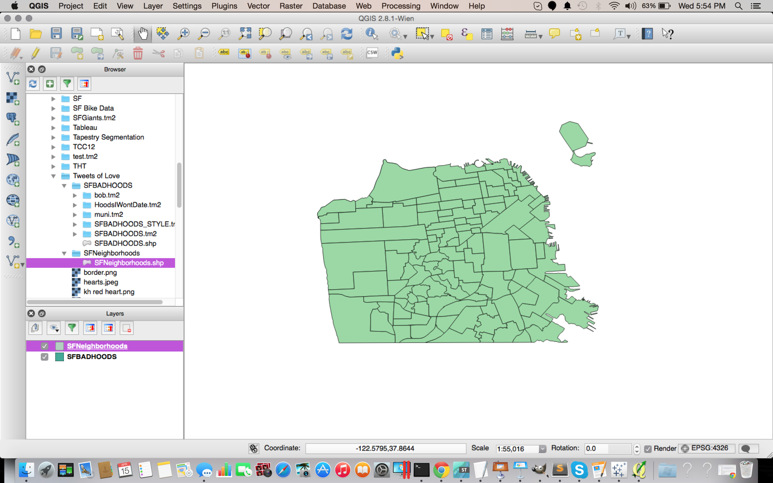
To look at, and play with my newly found shapefiles, I use an open source tool called QGIS.  If you need to, once you import your shapefiles, you can edit them so they are are just how you want them to be.   To do this, start a new project and from the "Layers" menu, select "Add Vector Layer.

Screen Shot 2015-04-15 at 5.57.07 PM

You should now see your shapefiles

Screen Shot 2015-04-15 at 5.54.20 PM

In my example, I wanted to be able to have a layer of neighborhoods where I would not consider dating be a map layer that I could turn on and off in Tableau.  As such, I only wanted to keep bad neighborhoods, and delete good ones.  This is not necessary before importing them into Mapbox, but it is also a great way to see any other attributes associated with the shapefiles like links to other information, attributes that group them together, or just plain see if what you downloaded was actually what you wanted.  You can also create your own shapes if you like, or add attributes to existing ones.
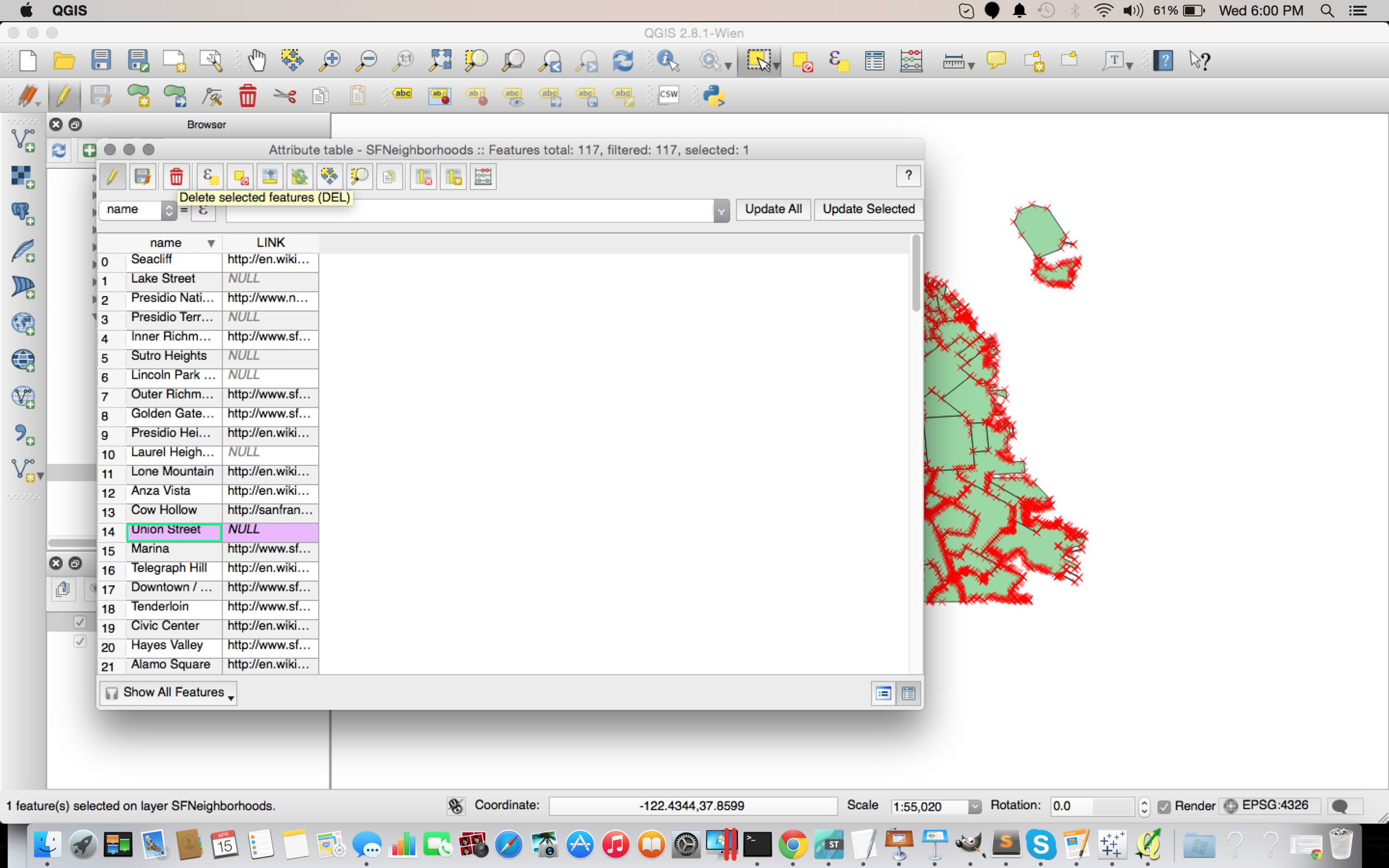
Screen Shot 2015-04-15 at 6.00.19 PM

Here is the updated map with only the neighborhoods that "I won't date in".

Screen Shot 2015-04-15 at 6.05.25 PM

Once you are finished editing your layers, select the “Layers” menu and then “save as”, and give your new shapefiles a name.   
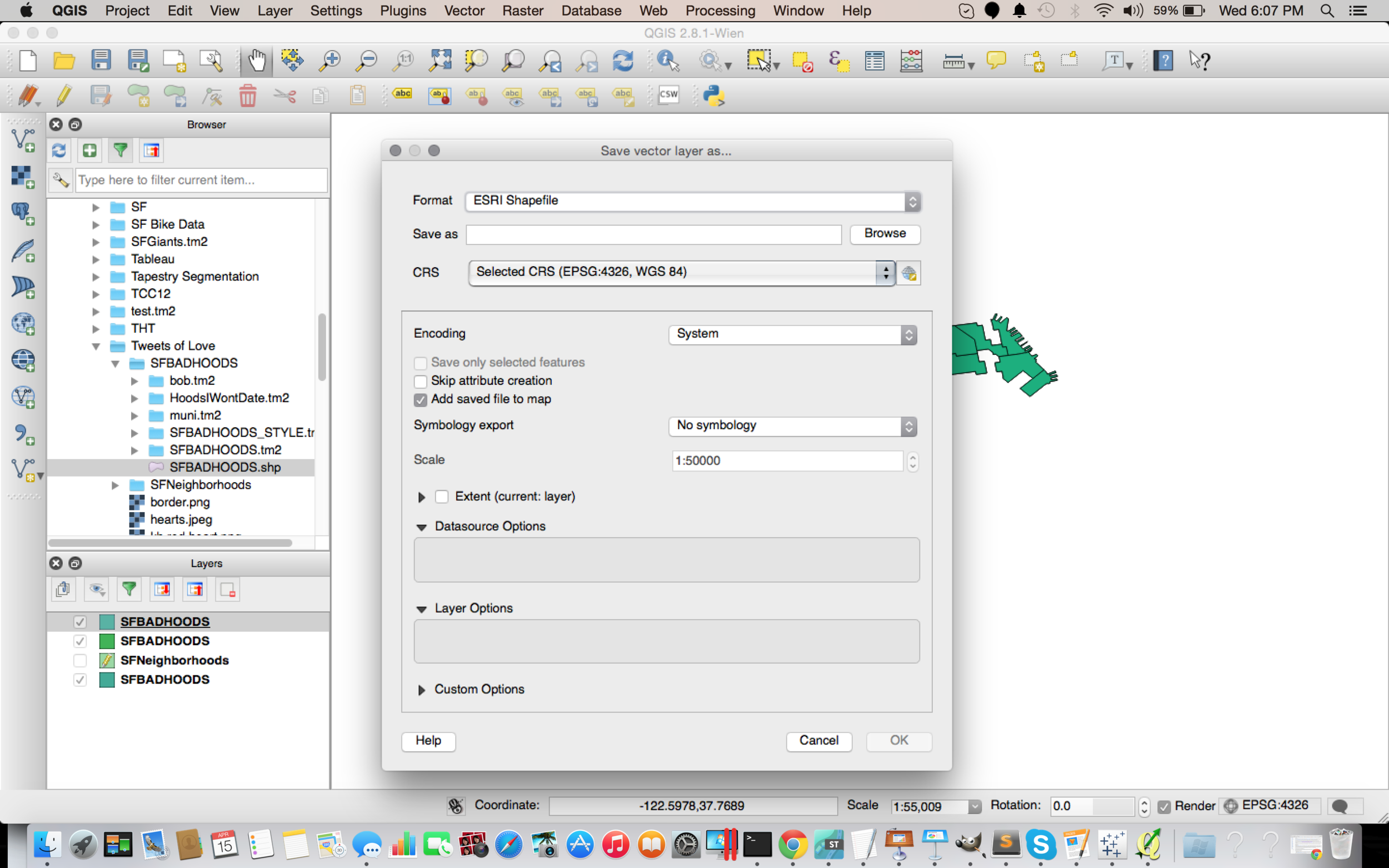
Screen Shot 2015-04-15 at 6.07.17 PM

Go to where they are saved and zip the folder that contains your new files.  The must be zipped for importing into Mapbox.

End of Optional Step and back to Mapbox

Go to mapbox.com and login to your account.  Click on “Data” in the upper left corner.  Then click on the “upload” button, so we can upload your data to Mapbox.  00

Browse to the file on your computer and upload it.  It will take a few moments to process the upload.  Once it is uploaded, click on the little copy icon to the right of the ID of your new data file.

000

In Mapbox Studio on the lower left corner, click on “Projects” and then “Create New”.  
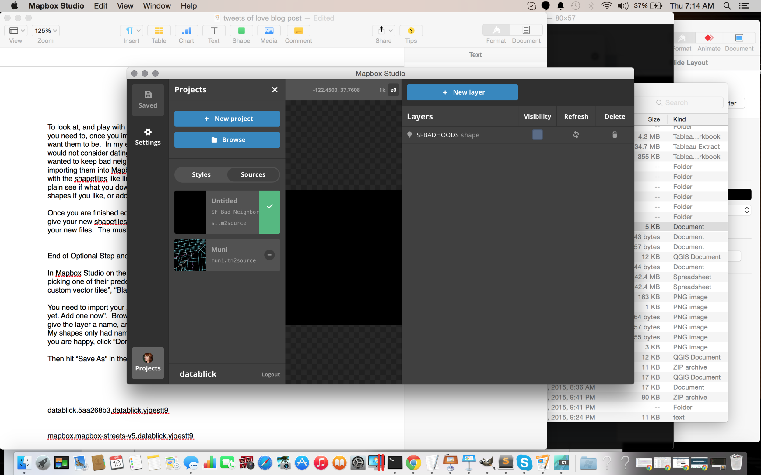
Screen Shot 2015-04-16 at 7.14.56 AM

Instead of picking one of their predefined styles, we will scroll down and use our newly created and uploaded source.   Use “Paste” to paste the ID and hit “Create”. 

Screen Shot 2015-04-16 at 7.26.22 AM

Oh, no?  Where did my shapes go?  Remember I was using San Francisco, and this showing a map of the world, so we need to search for SF, buy using the looking glass in the upper left corner.
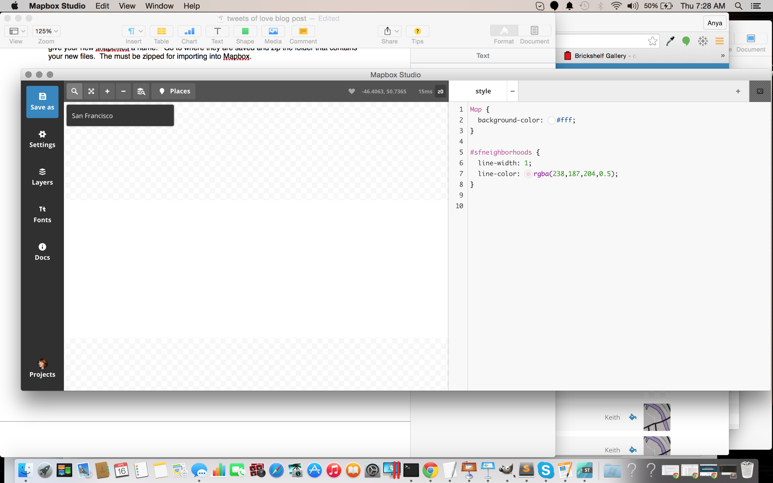
Screen Shot 2015-04-16 at 7.28.39 AM

Type in San Francisco, and a few results come back.  Select San Francisco, California, and then click on the looking glass again to hide it.  You should now see our San Francisco Neighborhoods.   Note your shapes may look different than mine if you did not use the Optional QGIS step to delete certain neighborhoods.  Either way, you will see a bunch of outlines of SF neighborhoods in Mapbox Studio and an area to the right where you can style them.

Screen Shot 2015-04-16 at 7.36.13 AMMake a simple change, like changing the color of the outline of the shapes by clicking on the small button to the right of “line-color” and picking a new color.  Alternately, you could just type in the color Hex value if you know what color you want.  You have to click “Save” in the upper right corner to see the change you just made.  Note, when you hit Save, your project is now saved with a new Folder on your local machine with the extension “.tm2source”.  This is where all the assets that make up your layer are stored. Screen Shot 2015-04-16 at 7.36.30 AM
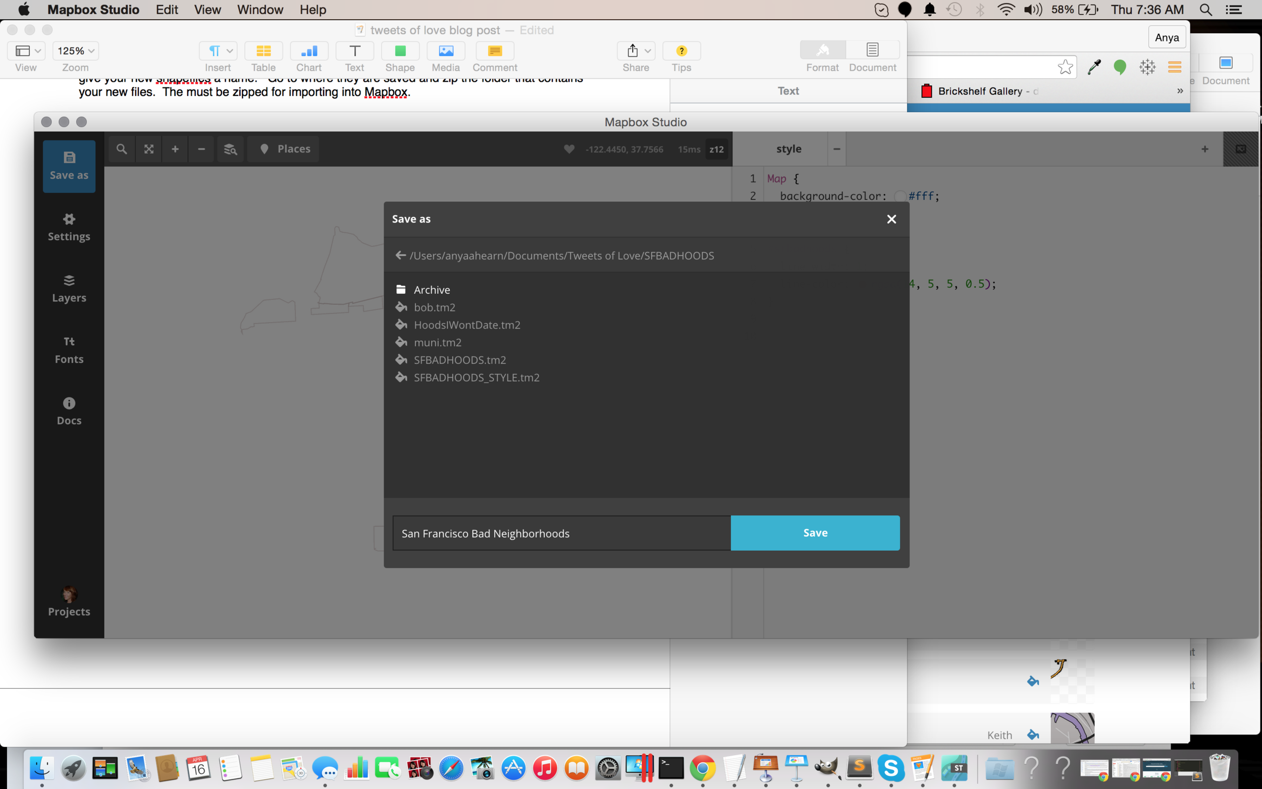
Back to your map layer, these are actually polygons, so we can fill them with a color if we like too.    For example, you could add the following to fill the shapes with hot pink.  You must hit "Save" to see any changes.

#sfbadhoods {

  line-width: 1;

  line-color: rgba(14, 5, 5, 0.5);

polygon-fill: #fd10cf;

}

If you want more information on styling your map elements, Mapbox has an online tutorial that walks through different options, or you can try anything that you might do using normal css formatting.  For the most part they work here too!  Go ahead..  “maps gone wild” time!  However, if you want to be lazy (it’s okay!) just use my style.

Hoods Style

Map {

/// background-color: #fff;

}

#SFNeighborhoods {

  line-width: 3;

  line-color: #000000;

  //polygon-fill: #d444dd;

// polygon-opacity: 0.4;

}

Screen Shot 2015-04-16 at 7.58.28 AM

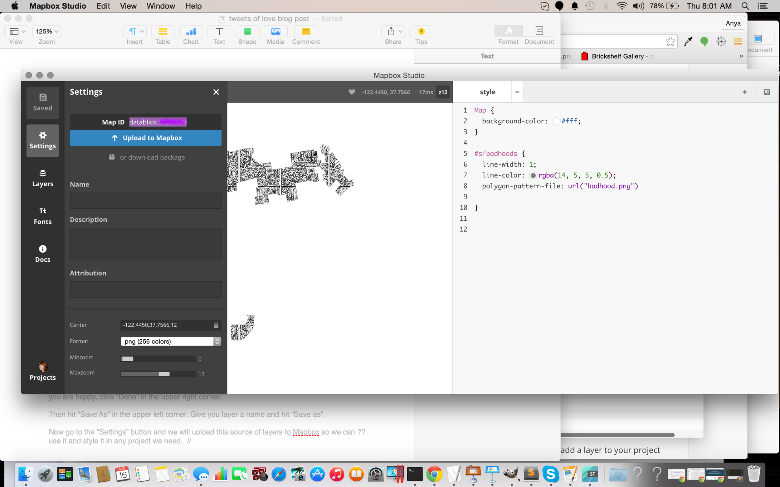
As I mentioned before, I wanted to make my Viz have the aesthetic of that Keith Haring painting, so I wanted to fill the polygons with some of his art.  To fill a polygon with a pattern or image you would using the following code which should point to an image file that you saved in your “My Project”.tm2source folder.  I used an image of a painting and referenced it as below after putting in my tm2source folder:

polygon-pattern-file: url(“/badhood.png");

Hit “Save” again, and you should now see the polygons filled with the painting.  Sweet!

Screen Shot 2015-04-16 at 7.58.38 AM 0

Once you have your layer styled the way you want it, then you need to upload it to Mapbox.  Click on “Settings”, and then Upload to Mapbox”.  Copy the ID that it returns, you will need this for your .tms file that Tableau will point to. 

Now go ahead and have some fun.  Add a few more shape layers, such as MUNI lines, water, bike lanes, police stations, whatever your heart desires.  I’ll wait for you…..

For this exercise, you may want to add a basic map to put these layers on top of, so go ahead and create a new project in Mapbox Studio, based it on one of their predefined styles and upload it to your account and copy the ID or just use the one that you made when you followed my previous post  http://datablick.com/2015/02/04/fast-and-fabulous-custom-maps-using-mapbox-in-tableau/  because of course you did that, right?

Are you ready?  You should now have at least 2 layers, the one you created based on an existing Mapbox style, and the one(s) you created with your own shapefiles.  Let’s get these layers into Tableau!

Creating a .tms with multiple layers

We are now going to create a .tms file to add to our map sources.    Here is an example of a .tms with just one layer.  The .tms file is just a little xml and can be edited in any text editor of your choice.  On windows I use Notepad ++ and on the Mac I use Sublime Text.
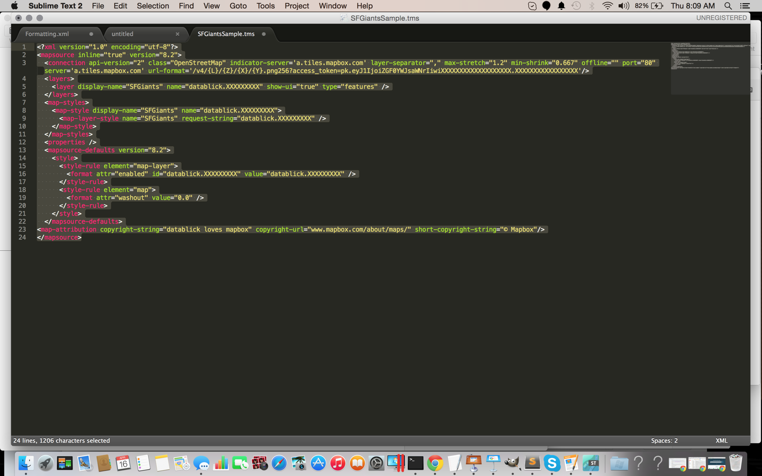
Screen Shot 2015-04-16 at 8.09.04 AM

The access_token is just your Mapbox ID and all the references to datablick.XXXXXXXXX are just pointing to your layer id in Mapbox.  How and what to change is explained in great detail in my previous post http://datablick.com/2015/02/04/fast-and-fabulous-custom-maps-using-mapbox-in-tableau/, so I wont go into that here.

The .tms with a multiple layers is not that much different.  There are really only 4 areas that need “find and replacing”, and you can easily add and delete more or fewer layers, but the basics are the same.  The order of the layers will determine which one is on top in the stacking order, so the top layer should be at the bottom of the list.

multiple layers (1)

  1. Replace the access_token key with your personal one from you mapbox.com account.
  2. Give each of your layers a name that you will use to turn it off and on in Tableau.
  3. Find and replace Map ID’s with yours
  4. Give a name to your fabulous group of layers

Now save it as a .tms file with a descriptive name, and put it in your c:\Documents\MyTableau Repository\Mapsources folder.

If you have Tableau open, then you need to close it and reopen it.

Build a basic viz that uses some location information.  I am of course going to use my Twitter, Tweets of Love data.  Use SuperStore if you want!  Just make sure it has some SF data.  Pick something like “Zip” and “Sales” and click “Show Me” to see it on a map.  Now go up to the “Map” menu and select “Background Maps” and then the name that you saved your .tms file as.
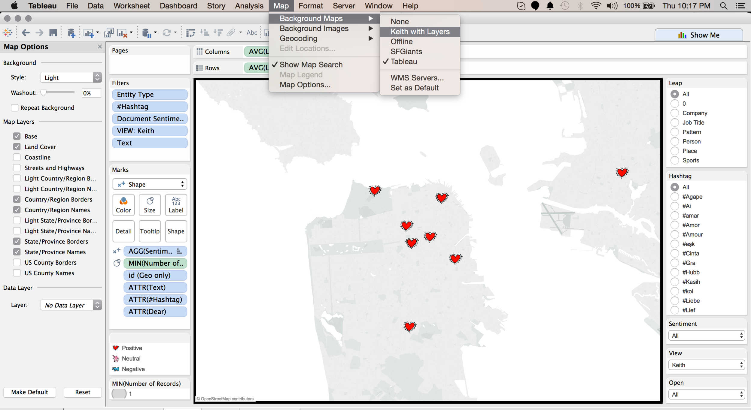
Screen Shot 2015-04-16 at 10.17.53 PM

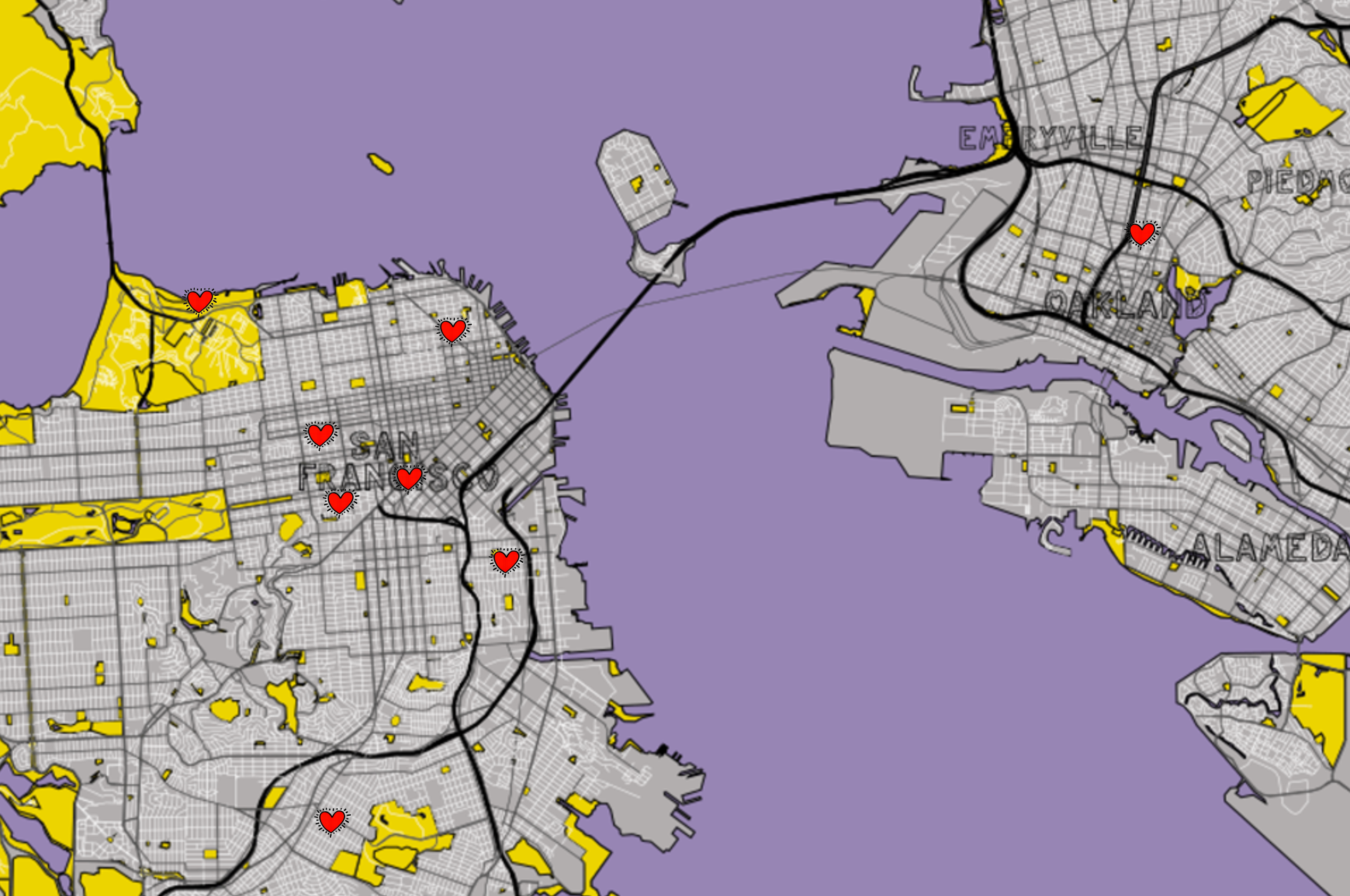
Go back to the “Map” menu and select “Map Options”.  On the left you will see the new layers you just added.  Toggle them on and off.  Each worksheet you have can have a different combination of the layers, or all the layers.  How fun is that!   Here is my map with the "Keith Haring" , MUNI and Neighborhoods layers.

Screen Shot 2015-04-16 at 10.18.05 PM

Here is my map with just the "Keith Haring" background map.
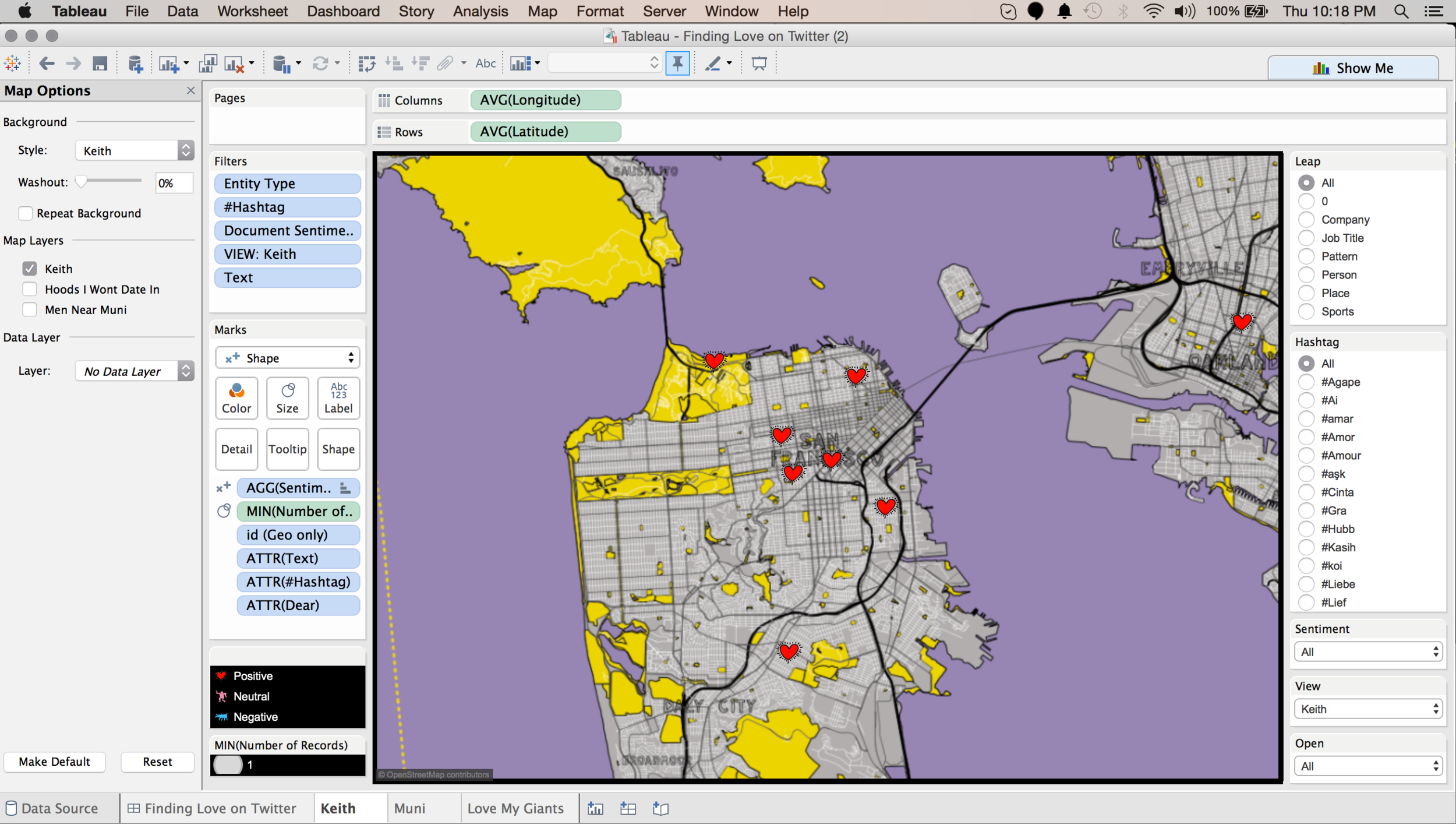
Screen Shot 2015-04-16 at 10.18.12 PM

Here is my map with the "SF MUNI" layer, making it much easier for me to see Tweets of Love that came from folks that are near a MUNI line.
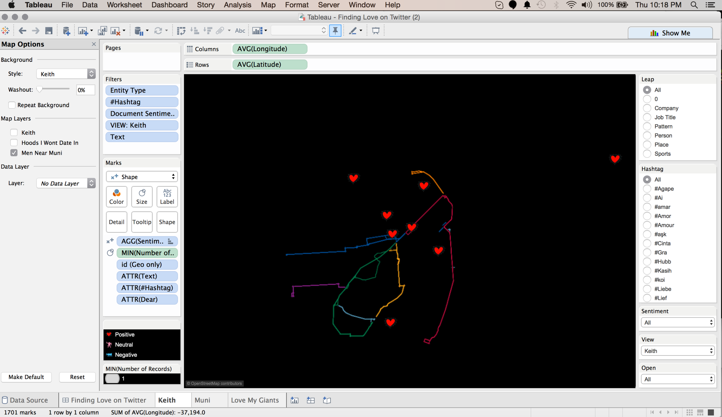
Screen Shot 2015-04-16 at 10.18.27 PM

Here is my map with the "Hoods I won't date in" layer, making it much easier for me to see Tweets of Love that are from folks in places I will go.  I was tempted to change my mind for him, because a day at the beach did sound kind of romantic.

Screen Shot 2015-04-16 at 10.18.44 PM

But then of course I found the Tweet that could only have come from my True Love (found using Twitter data).

Screen Shot 2015-04-16 at 10.18.57 PM

That’s all folks!  Have fun with custom map layers via Mapbox in Tableau!

Now back to Allan's blog post.  For the SFTUG, we decided to spice things up a bit and make my finding True Love using Twitter data a bit easier by adding Voice Control to the Viz.

Note - if you ever thought you didn’t do code, you do now girlfriend!  You just edited CSS and XML.  Congrats!  Go treat yourself to a little something something.

Circular and Hive Plot Network Graphing in Tableau by Chris DeMartini

17-Hive-3.png

I am delighted to host a guest blog post by Chris DeMartini on Network Graphing and Hive Plots on the fly in Tableau!  From Chris:

First off, want to send a big THANK YOU to Anya for the generosity and help she has provided, really for no reason at all, other than the fact that she is awesome and we are both San Francisco Giants fans.